

3.2 Constant Material and Geometry Parameters
43
In a similar way, we can write the approximation for node i + 1 and i − 1 as
d
2 u
dX 2
i+1
≈
u i+2 − 2u i+1 + u i
X 2
,
(3.11)
d
2 u
dX 2
i−1
≈
u i − 2u i−1 + u i−2
X 2
.
(3.12)
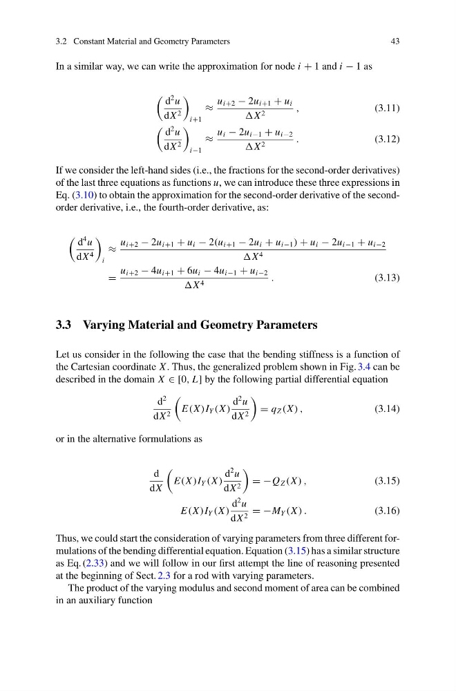
If we consider the left-hand sides (i.e., the fractions for the second-order derivatives)
of the last three equations as functions u, we can introduce these three expressions in
Eq. (3.10) to obtain the approximation for the second-order derivative of the secondorder derivative, i.e., the fourth-order derivative, as:
d
4 u
dX 4
i
≈
u i+2 − 2u i+1 + u i − 2(u i+1 − 2u i + u i−1 ) + u i − 2u i−1 + u i−2
X 4
=
u i+2 − 4u i+1 + 6u i − 4u i−1 + u i−2
X 4
.
(3.13)
3.3 Varying Material and Geometry Parameters
Let us consider in the following the case that the bending stiffness is a function of
the Cartesian coordinate X . Thus, the generalized problem shown in Fig. 3.4 can be
described in the domain X ∈ [0, L] by the following partial differential equation
d
2
dX 2
E(X )I Y (X )
d
2 u
dX 2
= q Z (X ) ,
(3.14)
or in the alternative formulations as
d
dX
E(X )I Y (X )
d
2 u
dX 2
= −Q Z (X ) ,
(3.15)
E(X )I Y (X )
d
2 u
dX 2 = −M Y (X ) .
(3.16)
Thus, we could start the consideration of varying parameters from three different formulations of the bending differential equation. Equation (3.15) has a similar structure
as Eq. (2.33) and we will follow in our first attempt the line of reasoning presented
at the beginning of Sect. 2.3 for a rod with varying parameters.
The product of the varying modulus and second moment of area can be combined
in an auxiliary function
43
In a similar way, we can write the approximation for node i + 1 and i − 1 as
d
2 u
dX 2
i+1
≈
u i+2 − 2u i+1 + u i
X 2
,
(3.11)
d
2 u
dX 2
i−1
≈
u i − 2u i−1 + u i−2
X 2
.
(3.12)
If we consider the left-hand sides (i.e., the fractions for the second-order derivatives)
of the last three equations as functions u, we can introduce these three expressions in
Eq. (3.10) to obtain the approximation for the second-order derivative of the secondorder derivative, i.e., the fourth-order derivative, as:
d
4 u
dX 4
i
≈
u i+2 − 2u i+1 + u i − 2(u i+1 − 2u i + u i−1 ) + u i − 2u i−1 + u i−2
X 4
=
u i+2 − 4u i+1 + 6u i − 4u i−1 + u i−2
X 4
.
(3.13)
3.3 Varying Material and Geometry Parameters
Let us consider in the following the case that the bending stiffness is a function of
the Cartesian coordinate X . Thus, the generalized problem shown in Fig. 3.4 can be
described in the domain X ∈ [0, L] by the following partial differential equation
d
2
dX 2
E(X )I Y (X )
d
2 u
dX 2
= q Z (X ) ,
(3.14)
or in the alternative formulations as
d
dX
E(X )I Y (X )
d
2 u
dX 2
= −Q Z (X ) ,
(3.15)
E(X )I Y (X )
d
2 u
dX 2 = −M Y (X ) .
(3.16)
Thus, we could start the consideration of varying parameters from three different formulations of the bending differential equation. Equation (3.15) has a similar structure
as Eq. (2.33) and we will follow in our first attempt the line of reasoning presented
at the beginning of Sect. 2.3 for a rod with varying parameters.
The product of the varying modulus and second moment of area can be combined
in an auxiliary function