

16
2 Investigation of Rods in the Elastic Range
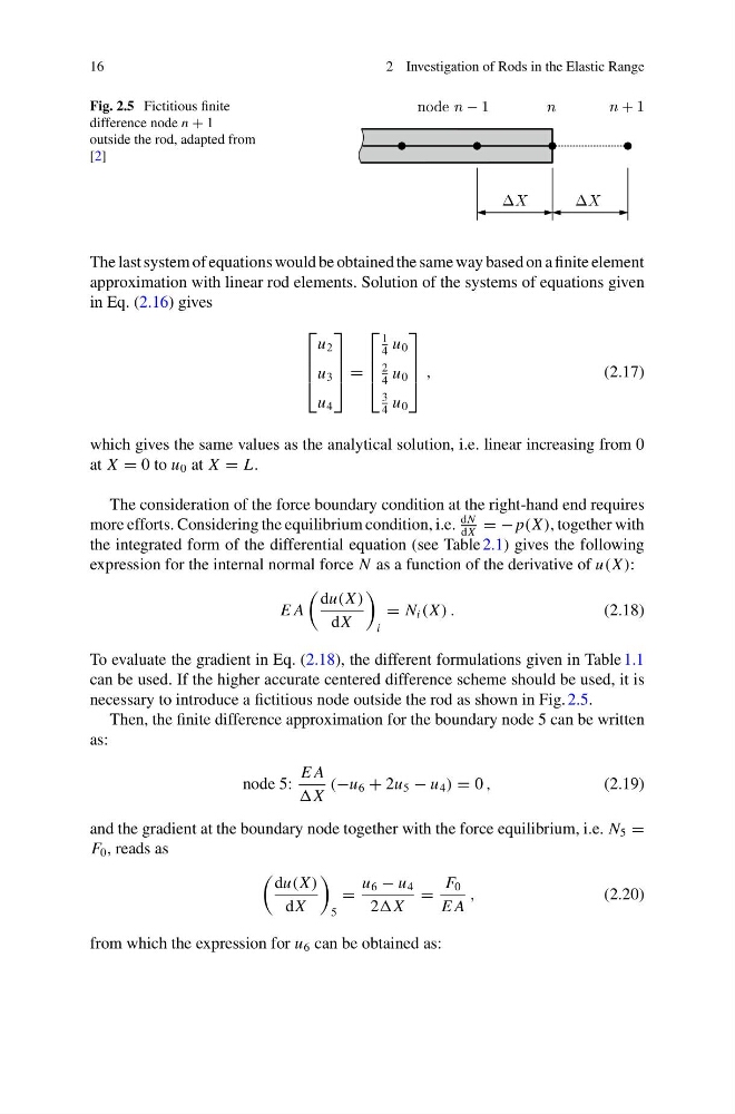
Fig. 2.5 Fictitious finite
difference node n + 1
outside the rod, adapted from
[2]
The last system of equations would be obtained the same way based on a finite element
approximation with linear rod elements. Solution of the systems of equations given
in Eq. (2.16) gives
⎡
⎢
⎢
⎣
u 2
u 3
u 4
⎤
⎥
⎥
⎦ =
⎡
⎢
⎢
⎣
1
4
u 0
2
4
u 0
3
4
u 0
⎤
⎥
⎥
⎦ ,
(2.17)
which gives the same values as the analytical solution, i.e. linear increasing from 0
at X = 0 to u 0 at X = L.
The consideration of the force boundary condition at the right-hand end requires
more efforts. Considering the equilibrium condition, i.e.
dN
dX
= −p(X ), together with
the integrated form of the differential equation (see Table 2.1) gives the following
expression for the internal normal force N as a function of the derivative of u(X ):
E A
du(X )
dX
i
= N i (X ) .
(2.18)
To evaluate the gradient in Eq. (2.18), the different formulations given in Table 1.1
can be used. If the higher accurate centered difference scheme should be used, it is
necessary to introduce a fictitious node outside the rod as shown in Fig. 2.5.
Then, the finite difference approximation for the boundary node 5 can be written
as:
node 5:
E A
(−u 6 + 2u 5 − u 4 ) = 0 ,
(2.19)
and the gradient at the boundary node together with the force equilibrium, i.e. N 5 =
F 0 , reads as
du(X )
dX
5
=
u 6 − u 4
2
=
F 0
E A
,
(2.20)
from which the expression for u 6 can be obtained as:
2 Investigation of Rods in the Elastic Range
Fig. 2.5 Fictitious finite
difference node n + 1
outside the rod, adapted from
[2]
The last system of equations would be obtained the same way based on a finite element
approximation with linear rod elements. Solution of the systems of equations given
in Eq. (2.16) gives
⎡
⎢
⎢
⎣
u 2
u 3
u 4
⎤
⎥
⎥
⎦ =
⎡
⎢
⎢
⎣
1
4
u 0
2
4
u 0
3
4
u 0
⎤
⎥
⎥
⎦ ,
(2.17)
which gives the same values as the analytical solution, i.e. linear increasing from 0
at X = 0 to u 0 at X = L.
The consideration of the force boundary condition at the right-hand end requires
more efforts. Considering the equilibrium condition, i.e.
dN
dX
= −p(X ), together with
the integrated form of the differential equation (see Table 2.1) gives the following
expression for the internal normal force N as a function of the derivative of u(X ):
E A
du(X )
dX
i
= N i (X ) .
(2.18)
To evaluate the gradient in Eq. (2.18), the different formulations given in Table 1.1
can be used. If the higher accurate centered difference scheme should be used, it is
necessary to introduce a fictitious node outside the rod as shown in Fig. 2.5.
Then, the finite difference approximation for the boundary node 5 can be written
as:
node 5:
E A
(−u 6 + 2u 5 − u 4 ) = 0 ,
(2.19)
and the gradient at the boundary node together with the force equilibrium, i.e. N 5 =
F 0 , reads as
du(X )
dX
5
=
u 6 − u 4
2
=
F 0
E A
,
(2.20)
from which the expression for u 6 can be obtained as: