

136
6 Answers to Supplementary Problems
⎡
⎢
⎢
⎣
2 0 0 0
−2 1 0 0
1 −2 1 0
0 1 −2 1
⎤
⎥
⎥
⎦
⎡
⎢
⎢
⎣
u 2
u 3
u 4
u 5
⎤
⎥
⎥
⎦ = −
X
2 F 0 L
E I Y
⎡
⎢
⎢
⎢
⎣
3
4
1
2
1
3
1
4
⎤
⎥
⎥
⎥
⎦
.
(6.133)
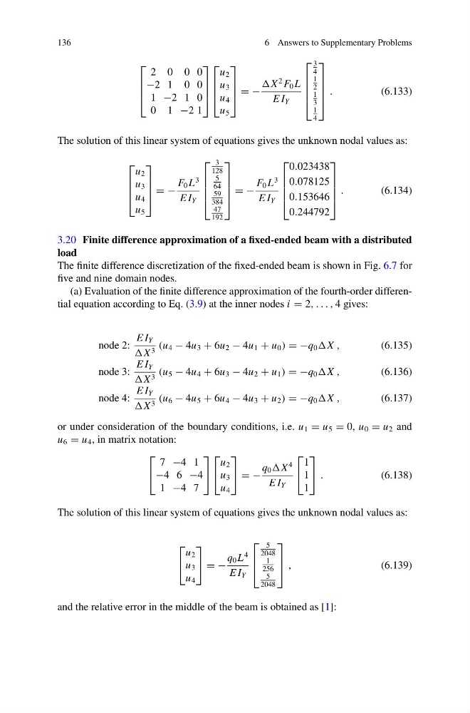
The solution of this linear system of equations gives the unknown nodal values as:
⎡
⎢
⎢
⎣
u 2
u 3
u 4
u 5
⎤
⎥
⎥
⎦ = −
F 0 L
3
E I Y
⎡
⎢
⎢
⎢
⎣
3
128
5
64
59
384
47
192
⎤
⎥
⎥
⎥
⎦
= −
F 0 L
3
E I Y
⎡
⎢
⎢
⎢
⎣
0.023438
0.078125
0.153646
0.244792
⎤
⎥
⎥
⎥
⎦
.
(6.134)
3.20 Finite difference approximation of a fixed-ended beam with a distributed
load
The finite difference discretization of the fixed-ended beam is shown in Fig. 6.7 for
five and nine domain nodes.
(a) Evaluation of the finite difference approximation of the fourth-order differential equation according to Eq. (3.9) at the inner nodes i = 2, . . . , 4 gives:
node 2:
E I Y
X 3 (u 4 − 4u 3 + 6u 2 − 4u 1 + u 0 ) = −q 0 X ,
(6.135)
node 3:
E I Y
X 3 (u 5 − 4u 4 + 6u 3 − 4u 2 + u 1 ) = −q 0 X ,
(6.136)
node 4:
E I Y
X 3 (u 6 − 4u 5 + 6u 4 − 4u 3 + u 2 ) = −q 0 X ,
(6.137)
or under consideration of the boundary conditions, i.e. u 1 = u 5 = 0, u 0 = u 2 and
u 6 = u 4 , in matrix notation:
⎡
⎣
7 −4 1
−4 6 −4
1 −4 7
⎤
⎦
⎡
⎣
u 2
u 3
u 4
⎤
⎦ = −
q 0 X
4
E I Y
⎡
⎣
1
1
1
⎤
⎦ .
(6.138)
The solution of this linear system of equations gives the unknown nodal values as:
⎡
⎣
u 2
u 3
u 4
⎤
⎦ = −
q 0 L
4
E I Y
⎡
⎢
⎣
5
2048
1
256
5
2048
⎤
⎥
⎦ ,
(6.139)
and the relative error in the middle of the beam is obtained as [1]:
6 Answers to Supplementary Problems
⎡
⎢
⎢
⎣
2 0 0 0
−2 1 0 0
1 −2 1 0
0 1 −2 1
⎤
⎥
⎥
⎦
⎡
⎢
⎢
⎣
u 2
u 3
u 4
u 5
⎤
⎥
⎥
⎦ = −
X
2 F 0 L
E I Y
⎡
⎢
⎢
⎢
⎣
3
4
1
2
1
3
1
4
⎤
⎥
⎥
⎥
⎦
.
(6.133)
The solution of this linear system of equations gives the unknown nodal values as:
⎡
⎢
⎢
⎣
u 2
u 3
u 4
u 5
⎤
⎥
⎥
⎦ = −
F 0 L
3
E I Y
⎡
⎢
⎢
⎢
⎣
3
128
5
64
59
384
47
192
⎤
⎥
⎥
⎥
⎦
= −
F 0 L
3
E I Y
⎡
⎢
⎢
⎢
⎣
0.023438
0.078125
0.153646
0.244792
⎤
⎥
⎥
⎥
⎦
.
(6.134)
3.20 Finite difference approximation of a fixed-ended beam with a distributed
load
The finite difference discretization of the fixed-ended beam is shown in Fig. 6.7 for
five and nine domain nodes.
(a) Evaluation of the finite difference approximation of the fourth-order differential equation according to Eq. (3.9) at the inner nodes i = 2, . . . , 4 gives:
node 2:
E I Y
X 3 (u 4 − 4u 3 + 6u 2 − 4u 1 + u 0 ) = −q 0 X ,
(6.135)
node 3:
E I Y
X 3 (u 5 − 4u 4 + 6u 3 − 4u 2 + u 1 ) = −q 0 X ,
(6.136)
node 4:
E I Y
X 3 (u 6 − 4u 5 + 6u 4 − 4u 3 + u 2 ) = −q 0 X ,
(6.137)
or under consideration of the boundary conditions, i.e. u 1 = u 5 = 0, u 0 = u 2 and
u 6 = u 4 , in matrix notation:
⎡
⎣
7 −4 1
−4 6 −4
1 −4 7
⎤
⎦
⎡
⎣
u 2
u 3
u 4
⎤
⎦ = −
q 0 X
4
E I Y
⎡
⎣
1
1
1
⎤
⎦ .
(6.138)
The solution of this linear system of equations gives the unknown nodal values as:
⎡
⎣
u 2
u 3
u 4
⎤
⎦ = −
q 0 L
4
E I Y
⎡
⎢
⎣
5
2048
1
256
5
2048
⎤
⎥
⎦ ,
(6.139)
and the relative error in the middle of the beam is obtained as [1]: