

124
6 Answers to Supplementary Problems
0
0 .5
1
1 .5
2
0
0.5
1
Normalized coordinate
X
L
Displacement u(X)
FDM
analytical solution
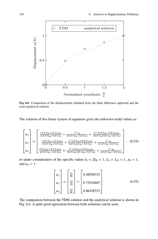
Fig. 6.6 Comparison of the displacements obtained from the finite difference approach and the
exact analytical solution
The solution of this linear system of equations gives the unknown nodal values as:
⎡
⎢
⎢
⎢
⎢
⎢
⎣
u 2
u 3
u 4
⎤
⎥
⎥
⎥
⎥
⎥
⎦
=
⎡
⎢
⎢
⎢
⎢
⎢
⎣
(3(E A) II +(E A) I) u 0
4(2(E A) II +2(E A) I )
+
L
2 p 0
4(2(E A) II +2(E A) I)
+
L
2 (5(E A) II +7(E A) I ) p 0
16(E A) I( 2(E A II +2(E A) I )
(3(E A) II +(E A) I )u0
2(2(E A) II +2(E A) I )
+
L
2 ((E A) II +3(E A) I ) p 0
8(E A) I( 2v II +2(E A) I )
+
L
2 p 0
2(2(E A) II +2(E A) I)
(7(E A) II +5(E A) I )u0
4(2(E A) II +2(E A) I )
+
L
2 ((E A) II +3(E A) I) p 0
16(E A) I (2(E A) II +2(E A) I)
+
L
2 p 0
4(2(E A) II +2(E A) I )
⎤
⎥
⎥
⎥
⎥
⎥
⎦
, (6.54)
or under consideration of the specific values k I = 2k II = 1, L I = L II = 1, p 0 = 1,
and u 0 = 1:
⎡
⎢
⎢
⎢
⎢
⎢
⎣
u 2
u 3
u 4
⎤
⎥
⎥
⎥
⎥
⎥
⎦
=
⎡
⎢
⎢
⎢
⎢
⎢
⎣
47
96
35
48
83
96
⎤
⎥
⎥
⎥
⎥
⎥
⎦
=
⎡
⎢
⎢
⎢
⎢
⎢
⎣
0.48958333
0.72916667
0.86458333
⎤
⎥
⎥
⎥
⎥
⎥
⎦
.
(6.55)
The comparison between the FDM solution and the analytical solution is shown in
Fig. 6.6. A quite good agreement between both solutions can be seen.
6 Answers to Supplementary Problems
0
0 .5
1
1 .5
2
0
0.5
1
Normalized coordinate
X
L
Displacement u(X)
FDM
analytical solution
Fig. 6.6 Comparison of the displacements obtained from the finite difference approach and the
exact analytical solution
The solution of this linear system of equations gives the unknown nodal values as:
⎡
⎢
⎢
⎢
⎢
⎢
⎣
u 2
u 3
u 4
⎤
⎥
⎥
⎥
⎥
⎥
⎦
=
⎡
⎢
⎢
⎢
⎢
⎢
⎣
(3(E A) II +(E A) I) u 0
4(2(E A) II +2(E A) I )
+
L
2 p 0
4(2(E A) II +2(E A) I)
+
L
2 (5(E A) II +7(E A) I ) p 0
16(E A) I( 2(E A II +2(E A) I )
(3(E A) II +(E A) I )u0
2(2(E A) II +2(E A) I )
+
L
2 ((E A) II +3(E A) I ) p 0
8(E A) I( 2v II +2(E A) I )
+
L
2 p 0
2(2(E A) II +2(E A) I)
(7(E A) II +5(E A) I )u0
4(2(E A) II +2(E A) I )
+
L
2 ((E A) II +3(E A) I) p 0
16(E A) I (2(E A) II +2(E A) I)
+
L
2 p 0
4(2(E A) II +2(E A) I )
⎤
⎥
⎥
⎥
⎥
⎥
⎦
, (6.54)
or under consideration of the specific values k I = 2k II = 1, L I = L II = 1, p 0 = 1,
and u 0 = 1:
⎡
⎢
⎢
⎢
⎢
⎢
⎣
u 2
u 3
u 4
⎤
⎥
⎥
⎥
⎥
⎥
⎦
=
⎡
⎢
⎢
⎢
⎢
⎢
⎣
47
96
35
48
83
96
⎤
⎥
⎥
⎥
⎥
⎥
⎦
=
⎡
⎢
⎢
⎢
⎢
⎢
⎣
0.48958333
0.72916667
0.86458333
⎤
⎥
⎥
⎥
⎥
⎥
⎦
.
(6.55)
The comparison between the FDM solution and the analytical solution is shown in
Fig. 6.6. A quite good agreement between both solutions can be seen.