

122
6 Answers to Supplementary Problems
0
0.17
0.33
0.5
0.67
0.83
1
0
0.1
0.2
0.3
Normalized coordinate
X
L
Normalized
displacement
u(X)
p
0 L 2
/(EA)
FDM
analytical solution
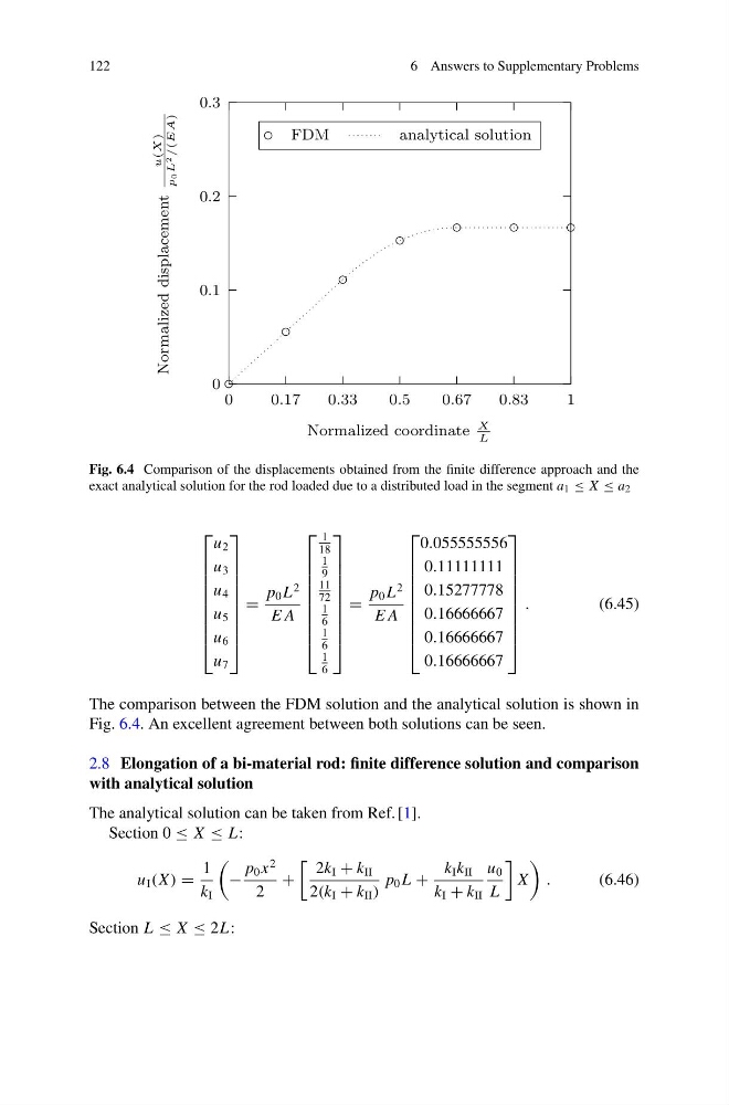
Fig. 6.4 Comparison of the displacements obtained from the finite difference approach and the
exact analytical solution for the rod loaded due to a distributed load in the segment a 1 ≤ X ≤ a 2
⎡
⎢
⎢
⎢
⎢
⎢
⎢
⎢
⎢
⎣
u 2
u 3
u 4
u 5
u 6
u 7
⎤
⎥
⎥
⎥
⎥
⎥
⎥
⎥
⎥
⎦
=
p 0 L
2
E A
⎡
⎢
⎢
⎢
⎢
⎢
⎢
⎢
⎢
⎣
1
18
1
9
11
72
1
6
1
6
1
6
⎤
⎥
⎥
⎥
⎥
⎥
⎥
⎥
⎥
⎦
=
p 0 L
2
E A
⎡
⎢
⎢
⎢
⎢
⎢
⎢
⎢
⎢
⎣
0.055555556
0.11111111
0.15277778
0.16666667
0.16666667
0.16666667
⎤
⎥
⎥
⎥
⎥
⎥
⎥
⎥
⎥
⎦
.
(6.45)
The comparison between the FDM solution and the analytical solution is shown in
Fig. 6.4. An excellent agreement between both solutions can be seen.
2.8 Elongation of a bi-material rod: finite difference solution and comparison
with analytical solution
The analytical solution can be taken from Ref. [1].
Section 0 ≤ X ≤ L:
u I (X ) =
1
k I
−
p 0 x
2
2
+
2k I + k II
2(k I + k II )
p 0 L +
k I k II
k I + k II
u 0
L
X
.
(6.46)
Section L ≤ X ≤ 2L:
6 Answers to Supplementary Problems
0
0.17
0.33
0.5
0.67
0.83
1
0
0.1
0.2
0.3
Normalized coordinate
X
L
Normalized
displacement
u(X)
p
0 L 2
/(EA)
FDM
analytical solution
Fig. 6.4 Comparison of the displacements obtained from the finite difference approach and the
exact analytical solution for the rod loaded due to a distributed load in the segment a 1 ≤ X ≤ a 2
⎡
⎢
⎢
⎢
⎢
⎢
⎢
⎢
⎢
⎣
u 2
u 3
u 4
u 5
u 6
u 7
⎤
⎥
⎥
⎥
⎥
⎥
⎥
⎥
⎥
⎦
=
p 0 L
2
E A
⎡
⎢
⎢
⎢
⎢
⎢
⎢
⎢
⎢
⎣
1
18
1
9
11
72
1
6
1
6
1
6
⎤
⎥
⎥
⎥
⎥
⎥
⎥
⎥
⎥
⎦
=
p 0 L
2
E A
⎡
⎢
⎢
⎢
⎢
⎢
⎢
⎢
⎢
⎣
0.055555556
0.11111111
0.15277778
0.16666667
0.16666667
0.16666667
⎤
⎥
⎥
⎥
⎥
⎥
⎥
⎥
⎥
⎦
.
(6.45)
The comparison between the FDM solution and the analytical solution is shown in
Fig. 6.4. An excellent agreement between both solutions can be seen.
2.8 Elongation of a bi-material rod: finite difference solution and comparison
with analytical solution
The analytical solution can be taken from Ref. [1].
Section 0 ≤ X ≤ L:
u I (X ) =
1
k I
−
p 0 x
2
2
+
2k I + k II
2(k I + k II )
p 0 L +
k I k II
k I + k II
u 0
L
X
.
(6.46)
Section L ≤ X ≤ 2L: