

120
6 Answers to Supplementary Problems
⎡
⎢
⎢
⎢
⎢
⎢
⎢
⎣
u 2
u 3
u 4
u 5
u 6
⎤
⎥
⎥
⎥
⎥
⎥
⎥
⎦
=
p 0 L
2
E A
⎡
⎢
⎢
⎢
⎢
⎢
⎢
⎣
49
216
37
108
25
72
31
108
37
216
⎤
⎥
⎥
⎥
⎥
⎥
⎥
⎦
.
(6.28)
2.7 Elongation of a rod due to distributed load
The analytical solution can be taken from Ref. [1].
Section 0 ≤ X ≤ a 1 :
u I (X ) =
p 0 (a 2 − a 1 )
E A
× X
=
1
3
×
p 0 L
2
E A
×
X
L
.
(6.29)
Section a 1 ≤ X ≤ a 2 :
u II (X ) =
p 0
E A
−
1
2
(X − a 1 )
2
+ (a 2 − a 1 )X
=
p 0 L
2
E A
−
1
2
X
L
−
1
3
2
+
1
3
×
X
L
.
(6.30)
Section a 2 ≤ X ≤ L:
u III (X ) =
p 0
E A
−
1
2
2L
3
− a 1
2
+ (a 2 − a 1 )
2L
3
=
1
6
×
p 0 L
2
E A
= const .
(6.31)
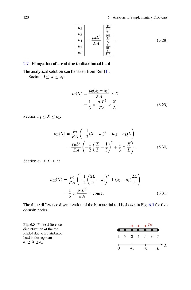
The finite difference discretization of the bi-material rod is shown in Fig. 6.3 for five
domain nodes.
Fig. 6.3 Finite difference
discretization of the rod
loaded due to a distributed
load in the segment
a 1 ≤ X ≤ a 2
6 Answers to Supplementary Problems
⎡
⎢
⎢
⎢
⎢
⎢
⎢
⎣
u 2
u 3
u 4
u 5
u 6
⎤
⎥
⎥
⎥
⎥
⎥
⎥
⎦
=
p 0 L
2
E A
⎡
⎢
⎢
⎢
⎢
⎢
⎢
⎣
49
216
37
108
25
72
31
108
37
216
⎤
⎥
⎥
⎥
⎥
⎥
⎥
⎦
.
(6.28)
2.7 Elongation of a rod due to distributed load
The analytical solution can be taken from Ref. [1].
Section 0 ≤ X ≤ a 1 :
u I (X ) =
p 0 (a 2 − a 1 )
E A
× X
=
1
3
×
p 0 L
2
E A
×
X
L
.
(6.29)
Section a 1 ≤ X ≤ a 2 :
u II (X ) =
p 0
E A
−
1
2
(X − a 1 )
2
+ (a 2 − a 1 )X
=
p 0 L
2
E A
−
1
2
X
L
−
1
3
2
+
1
3
×
X
L
.
(6.30)
Section a 2 ≤ X ≤ L:
u III (X ) =
p 0
E A
−
1
2
2L
3
− a 1
2
+ (a 2 − a 1 )
2L
3
=
1
6
×
p 0 L
2
E A
= const .
(6.31)
The finite difference discretization of the bi-material rod is shown in Fig. 6.3 for five
domain nodes.
Fig. 6.3 Finite difference
discretization of the rod
loaded due to a distributed
load in the segment
a 1 ≤ X ≤ a 2