

6.2 Answers for Problems from Chap. 2
117
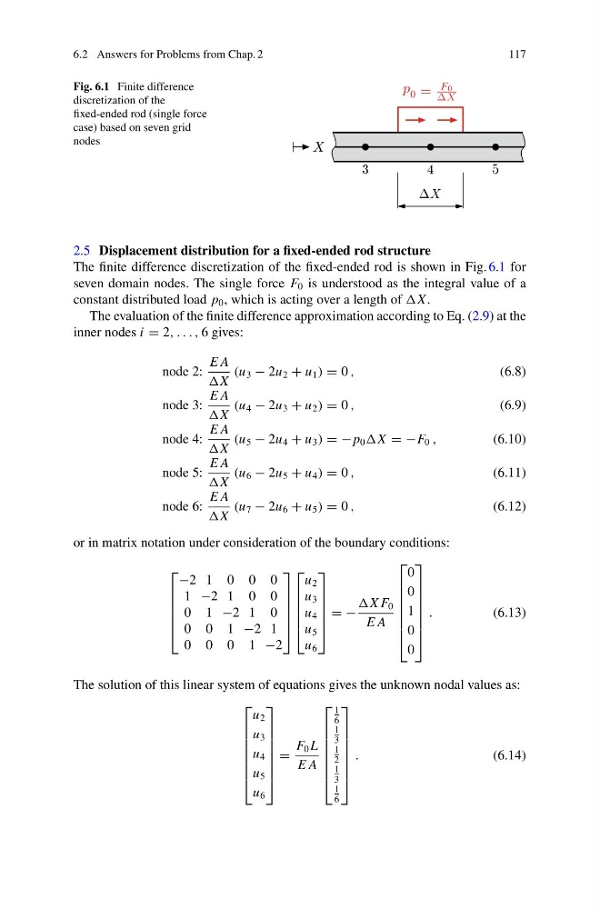
Fig. 6.1 Finite difference
discretization of the
fixed-ended rod (single force
case) based on seven grid
nodes
2.5 Displacement distribution for a fixed-ended rod structure
The finite difference discretization of the fixed-ended rod is shown in Fig. 6.1 for
seven domain nodes. The single force F 0 is understood as the integral value of a
constant distributed load p 0 , which is acting over a length of .
The evaluation of the finite difference approximation according to Eq. (2.9) at the
inner nodes i = 2, . . . , 6 gives:
node 2:
E A
(u 3 − 2u 2 + u 1 ) = 0 ,
(6.8)
node 3:
E A
X
(u 4 − 2u 3 + u 2 ) = 0 ,
(6.9)
node 4:
E A
X
(u 5 − 2u 4 + u 3 ) = −p 0 = −F 0 ,
(6.10)
node 5:
E A
X
(u 6 − 2u 5 + u 4 ) = 0 ,
(6.11)
node 6:
E A
X
(u 7 − 2u 6 + u 5 ) = 0 ,
(6.12)
or in matrix notation under consideration of the boundary conditions:
⎡
⎢
⎢
⎢
⎢
⎣
−2 1 0 0 0
1 −2 1 0 0
0 1 −2 1 0
0 0 1 −2 1
0 0 0 1 −2
⎤
⎥
⎥
⎥
⎥
⎦
⎡
⎢
⎢
⎢
⎢
⎣
u 2
u 3
u 4
u 5
u 6
⎤
⎥
⎥
⎥
⎥
⎦
= −
X F 0
E A
⎡
⎢
⎢
⎢
⎢
⎢
⎢
⎣
0
0
1
0
0
⎤
⎥
⎥
⎥
⎥
⎥
⎥
⎦
.
(6.13)
The solution of this linear system of equations gives the unknown nodal values as:
⎡
⎢
⎢
⎢
⎢
⎢
⎢
⎣
u 2
u 3
u 4
u 5
u 6
⎤
⎥
⎥
⎥
⎥
⎥
⎥
⎦
=
F 0 L
E A
⎡
⎢
⎢
⎢
⎢
⎢
⎢
⎣
1
6
1
3
1
2
1
3
1
6
⎤
⎥
⎥
⎥
⎥
⎥
⎥
⎦
.
(6.14)
117
Fig. 6.1 Finite difference
discretization of the
fixed-ended rod (single force
case) based on seven grid
nodes
2.5 Displacement distribution for a fixed-ended rod structure
The finite difference discretization of the fixed-ended rod is shown in Fig. 6.1 for
seven domain nodes. The single force F 0 is understood as the integral value of a
constant distributed load p 0 , which is acting over a length of .
The evaluation of the finite difference approximation according to Eq. (2.9) at the
inner nodes i = 2, . . . , 6 gives:
node 2:
E A
(u 3 − 2u 2 + u 1 ) = 0 ,
(6.8)
node 3:
E A
X
(u 4 − 2u 3 + u 2 ) = 0 ,
(6.9)
node 4:
E A
X
(u 5 − 2u 4 + u 3 ) = −p 0 = −F 0 ,
(6.10)
node 5:
E A
X
(u 6 − 2u 5 + u 4 ) = 0 ,
(6.11)
node 6:
E A
X
(u 7 − 2u 6 + u 5 ) = 0 ,
(6.12)
or in matrix notation under consideration of the boundary conditions:
⎡
⎢
⎢
⎢
⎢
⎣
−2 1 0 0 0
1 −2 1 0 0
0 1 −2 1 0
0 0 1 −2 1
0 0 0 1 −2
⎤
⎥
⎥
⎥
⎥
⎦
⎡
⎢
⎢
⎢
⎢
⎣
u 2
u 3
u 4
u 5
u 6
⎤
⎥
⎥
⎥
⎥
⎦
= −
X F 0
E A
⎡
⎢
⎢
⎢
⎢
⎢
⎢
⎣
0
0
1
0
0
⎤
⎥
⎥
⎥
⎥
⎥
⎥
⎦
.
(6.13)
The solution of this linear system of equations gives the unknown nodal values as:
⎡
⎢
⎢
⎢
⎢
⎢
⎢
⎣
u 2
u 3
u 4
u 5
u 6
⎤
⎥
⎥
⎥
⎥
⎥
⎥
⎦
=
F 0 L
E A
⎡
⎢
⎢
⎢
⎢
⎢
⎢
⎣
1
6
1
3
1
2
1
3
1
6
⎤
⎥
⎥
⎥
⎥
⎥
⎥
⎦
.
(6.14)