

108
5 Consideration of Euler–Bernoulli Beams with Plastic Material Behavior
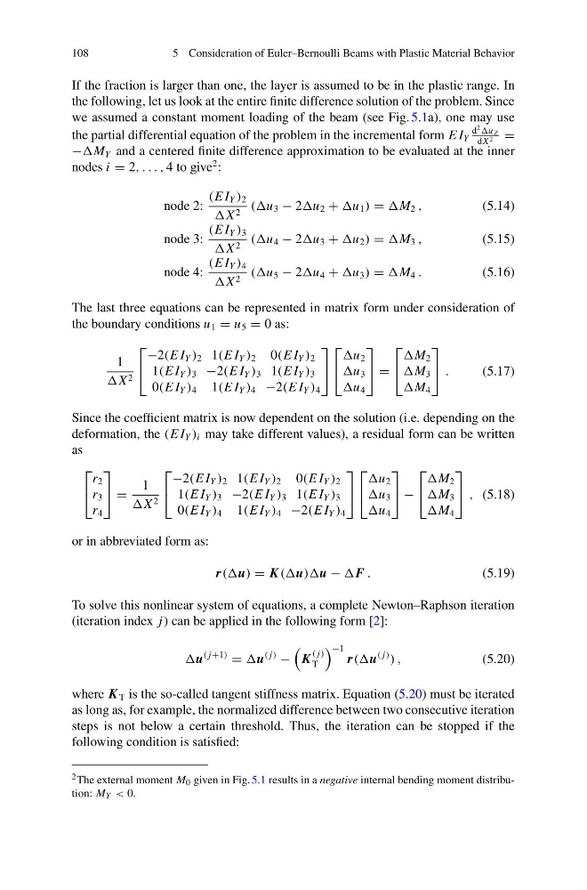
If the fraction is larger than one, the layer is assumed to be in the plastic range. In
the following, let us look at the entire finite difference solution of the problem. Since
we assumed a constant moment loading of the beam (see Fig. 5.1a), one may use
the partial differential equation of the problem in the incremental form E I Y
d
2 u Z
dX 2 =
−M Y and a centered finite difference approximation to be evaluated at the inner
nodes i = 2, . . . , 4 to give
2 :
node 2:
(E I Y ) 2
X 2 (u 3 − 2u 2 + u 1 ) = M 2 ,
(5.14)
node 3:
(E I Y ) 3
X 2 (u 4 − 2u 3 + u 2 ) = M 3 ,
(5.15)
node 4:
(E I Y ) 4
X 2 (u 5 − 2u 4 + u 3 ) = M 4 .
(5.16)
The last three equations can be represented in matrix form under consideration of
the boundary conditions u 1 = u 5 = 0 as:
1
X 2
⎡
⎣
−2(E I Y ) 2 1(E I Y ) 2 0(E I Y ) 2
1(E I Y ) 3 −2(E I Y ) 3 1(E I Y ) 3
0(E I Y ) 4 1(E I Y ) 4 −2(E I Y ) 4
⎤
⎦
⎡
⎣
u 2
u 3
u 4
⎤
⎦ =
⎡
⎣
M 2
M 3
M 4
⎤
⎦ .
(5.17)
Since the coefficient matrix is now dependent on the solution (i.e. depending on the
deformation, the (E I Y ) i may take different values), a residual form can be written
as
⎡
⎣
r 2
r 3
r 4
⎤
⎦ =
1
X 2
⎡
⎣
−2(E I Y ) 2 1(E I Y ) 2 0(E I Y ) 2
1(E I Y ) 3 −2(E I Y ) 3 1(E I Y ) 3
0(E I Y ) 4 1(E I Y ) 4 −2(E I Y ) 4
⎤
⎦
⎡
⎣
u 2
u 3
u 4
⎤
⎦ −
⎡
⎣
M 2
M 3
M 4
⎤
⎦ , (5.18)
or in abbreviated form as:
r((u) = K ((u))u − F .
(5.19)
To solve this nonlinear system of equations, a complete Newton–Raphson iteration
(iteration index j) can be applied in the following form [2]:
u
( j+1)
= u
( j)
−
K
( j)
T
−1
r((u
( j)
) ,
(5.20)
where K T is the so-called tangent stiffness matrix. Equation (5.20) must be iterated
as long as, for example, the normalized difference between two consecutive iteration
steps is not below a certain threshold. Thus, the iteration can be stopped if the
following condition is satisfied:
2 The external moment M 0 given in Fig. 5.1 results in a negative internal bending moment distribution: M Y < 0.
5 Consideration of Euler–Bernoulli Beams with Plastic Material Behavior
If the fraction is larger than one, the layer is assumed to be in the plastic range. In
the following, let us look at the entire finite difference solution of the problem. Since
we assumed a constant moment loading of the beam (see Fig. 5.1a), one may use
the partial differential equation of the problem in the incremental form E I Y
d
2 u Z
dX 2 =
−M Y and a centered finite difference approximation to be evaluated at the inner
nodes i = 2, . . . , 4 to give
2 :
node 2:
(E I Y ) 2
X 2 (u 3 − 2u 2 + u 1 ) = M 2 ,
(5.14)
node 3:
(E I Y ) 3
X 2 (u 4 − 2u 3 + u 2 ) = M 3 ,
(5.15)
node 4:
(E I Y ) 4
X 2 (u 5 − 2u 4 + u 3 ) = M 4 .
(5.16)
The last three equations can be represented in matrix form under consideration of
the boundary conditions u 1 = u 5 = 0 as:
1
X 2
⎡
⎣
−2(E I Y ) 2 1(E I Y ) 2 0(E I Y ) 2
1(E I Y ) 3 −2(E I Y ) 3 1(E I Y ) 3
0(E I Y ) 4 1(E I Y ) 4 −2(E I Y ) 4
⎤
⎦
⎡
⎣
u 2
u 3
u 4
⎤
⎦ =
⎡
⎣
M 2
M 3
M 4
⎤
⎦ .
(5.17)
Since the coefficient matrix is now dependent on the solution (i.e. depending on the
deformation, the (E I Y ) i may take different values), a residual form can be written
as
⎡
⎣
r 2
r 3
r 4
⎤
⎦ =
1
X 2
⎡
⎣
−2(E I Y ) 2 1(E I Y ) 2 0(E I Y ) 2
1(E I Y ) 3 −2(E I Y ) 3 1(E I Y ) 3
0(E I Y ) 4 1(E I Y ) 4 −2(E I Y ) 4
⎤
⎦
⎡
⎣
u 2
u 3
u 4
⎤
⎦ −
⎡
⎣
M 2
M 3
M 4
⎤
⎦ , (5.18)
or in abbreviated form as:
r((u) = K ((u))u − F .
(5.19)
To solve this nonlinear system of equations, a complete Newton–Raphson iteration
(iteration index j) can be applied in the following form [2]:
u
( j+1)
= u
( j)
−
K
( j)
T
−1
r((u
( j)
) ,
(5.20)
where K T is the so-called tangent stiffness matrix. Equation (5.20) must be iterated
as long as, for example, the normalized difference between two consecutive iteration
steps is not below a certain threshold. Thus, the iteration can be stopped if the
following condition is satisfied:
2 The external moment M 0 given in Fig. 5.1 results in a negative internal bending moment distribution: M Y < 0.