

90
4 Investigation of Timoshenko Beams in the Elastic Range
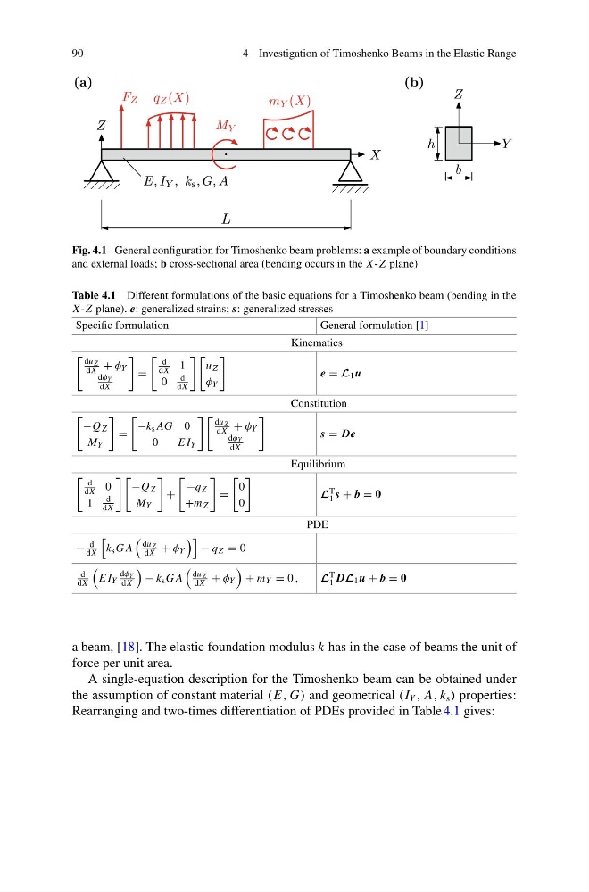
Fig. 4.1 General configuration for Timoshenko beam problems: a example of boundary conditions
and external loads; b cross-sectional area (bending occurs in the X -Z plane)
Table 4.1 Different formulations of the basic equations for a Timoshenko beam (bending in the
X -Z plane). e: generalized strains; s: generalized stresses
Specific formulation
General formulation [1]
Kinematics
du Z
dX + φ Y
dφ Y
dX
=
d
dX 1
0
d
dX
u Z
φ Y
e = L 1 u
Constitution
−Q Z
M Y
=
−k s AG 0
0
E I Y
du Z
dX + φ Y
dφ Y
dX
s = De
Equilibrium
d
dX 0
1
d
dX
−Q Z
M Y
+
−q Z
+m Z
=
0
0
L T
1 s + b = 0
PDE
−
d
dX
k s G A
du Z
dX + φ Y
− q Z = 0
d
dX
E I Y
dφ Y
dX
− k s G A
du Z
dX + φ Y
+ m Y = 0 ,
L T
1 DL 1 u + b = 0
a beam, [18]. The elastic foundation modulus k has in the case of beams the unit of
force per unit area.
A single-equation description for the Timoshenko beam can be obtained under
the assumption of constant material (E, G) and geometrical (I Y , A, k s ) properties:
Rearranging and two-times differentiation of PDEs provided in Table 4.1 gives:
4 Investigation of Timoshenko Beams in the Elastic Range
Fig. 4.1 General configuration for Timoshenko beam problems: a example of boundary conditions
and external loads; b cross-sectional area (bending occurs in the X -Z plane)
Table 4.1 Different formulations of the basic equations for a Timoshenko beam (bending in the
X -Z plane). e: generalized strains; s: generalized stresses
Specific formulation
General formulation [1]
Kinematics
du Z
dX + φ Y
dφ Y
dX
=
d
dX 1
0
d
dX
u Z
φ Y
e = L 1 u
Constitution
−Q Z
M Y
=
−k s AG 0
0
E I Y
du Z
dX + φ Y
dφ Y
dX
s = De
Equilibrium
d
dX 0
1
d
dX
−Q Z
M Y
+
−q Z
+m Z
=
0
0
L T
1 s + b = 0
PDE
−
d
dX
k s G A
du Z
dX + φ Y
− q Z = 0
d
dX
E I Y
dφ Y
dX
− k s G A
du Z
dX + φ Y
+ m Y = 0 ,
L T
1 DL 1 u + b = 0
a beam, [18]. The elastic foundation modulus k has in the case of beams the unit of
force per unit area.
A single-equation description for the Timoshenko beam can be obtained under
the assumption of constant material (E, G) and geometrical (I Y , A, k s ) properties:
Rearranging and two-times differentiation of PDEs provided in Table 4.1 gives: