

6.1 Basic Concepts and Formulae
315
Inverse transformations
x = γ (x
+ νt
)
(6.12)
y = y
(6.13)
z = z
(6.14)
t = γ
t
+
νx
c 2
(6.15)
with
γ =
1
(1 − β 2 )
=
1
√
(1 − ν 2 /c 2 )
(6.16)
and
β =
ν
c
(6.17)
Transformation matrix
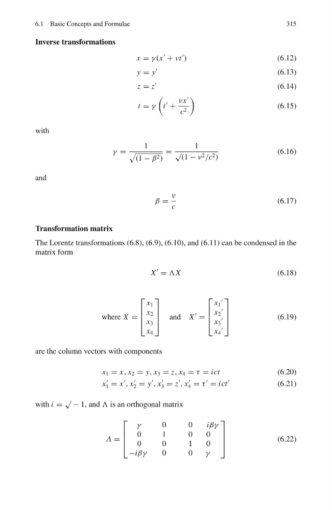
The Lorentz transformations (6.8), (6.9), (6.10), and (6.11) can be condensed in the
matrix form
X
= ΛX
(6.18)
where X =
⎡
⎢
⎢
⎣
x 1
x 2
x 3
x 4
⎤
⎥
⎥
⎦ and X
=
⎡
⎢
⎢
⎣
x 1
x 2
x 3
x 4
⎤
⎥
⎥
⎦
(6.19)
are the column vectors with components
x 1 = x, x 2 = y, x 3 = z, x 4 = τ = ict
(6.20)
x
1 = x
, x
2 = y
, x
3 = z
, x
4 = τ
= ict
(6.21)
with i =
√ − 1, and Λ is an orthogonal matrix
Λ =
⎡
⎢
⎢
⎣
γ
0
0
iβγ
0
1
0
0
0
0
1
0
−iβγ
0
0
γ
⎤
⎥
⎥
⎦
(6.22)
315
Inverse transformations
x = γ (x
+ νt
)
(6.12)
y = y
(6.13)
z = z
(6.14)
t = γ
t
+
νx
c 2
(6.15)
with
γ =
1
(1 − β 2 )
=
1
√
(1 − ν 2 /c 2 )
(6.16)
and
β =
ν
c
(6.17)
Transformation matrix
The Lorentz transformations (6.8), (6.9), (6.10), and (6.11) can be condensed in the
matrix form
X
= ΛX
(6.18)
where X =
⎡
⎢
⎢
⎣
x 1
x 2
x 3
x 4
⎤
⎥
⎥
⎦ and X
=
⎡
⎢
⎢
⎣
x 1
x 2
x 3
x 4
⎤
⎥
⎥
⎦
(6.19)
are the column vectors with components
x 1 = x, x 2 = y, x 3 = z, x 4 = τ = ict
(6.20)
x
1 = x
, x
2 = y
, x
3 = z
, x
4 = τ
= ict
(6.21)
with i =
√ − 1, and Λ is an orthogonal matrix
Λ =
⎡
⎢
⎢
⎣
γ
0
0
iβγ
0
1
0
0
0
0
1
0
−iβγ
0
0
γ
⎤
⎥
⎥
⎦
(6.22)