

168
3 Quantum Mechanics – II
1
sin θ
∂
∂θ
sin θ
d f
dθ
+ λ f (θ ) = 0
( 2 )
d
dθ
=
d
dμ
·
dμ
dθ
= − sin θ
d
dμ
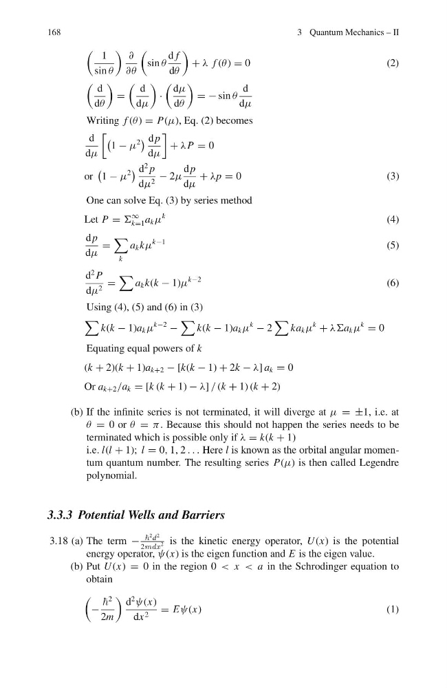
Writing f (θ ) = P(μ), Eq. (2) becomes
d
dμ
1 − μ
2
d p
dμ
+ λP = 0
or
1 − μ
2
d
2 p
dμ 2 − 2μ
d p
dμ
+ λp = 0
( 3 )
One can solve Eq. (3) by series method
Let P = Σ
∞
k=1 a k μ
k
(4)
d p
dμ
=
k
a k kμ
k−1
(5)
d
2 P
dμ 2 =
a k k(k − 1)μ
k−2
(6)
Using (4), (5) and (6) in (3)
k(k − 1)a k μ
k−2
−
k(k − 1)a k μ
k
− 2
ka k μ
k
+ λΣa k μ
k
= 0
Equating equal powers of k
(k + 2)(k + 1)a k+2 − [k(k − 1) + 2k − λ] a k = 0
Or a k+2 /a k = [k (k + 1) − λ] / (k + 1) (k + 2)
(b) If the infinite series is not terminated, it will diverge at μ = ±1, i.e. at
θ = 0 or θ = π. Because this should not happen the series needs to be
terminated which is possible only if λ = k(k + 1)
i.e. l(l + 1); l = 0, 1, 2 . . . Here l is known as the orbital angular momentum quantum number. The resulting series P(μ) is then called Legendre
polynomial.
3.3.3 Potential Wells and Barriers
3.18 (a) The term −
2 d
2
2mdx
2 is the kinetic energy operator, U (x) is the potential
energy operator, ψ(x) is the eigen function and E is the eigen value.
(b) Put U (x) = 0 in the region 0 < x < a in the Schrodinger equation to
obtain
−
2
2m
d
2
ψ(x)
dx 2 = Eψ(x)
( 1 )
3 Quantum Mechanics – II
1
sin θ
∂
∂θ
sin θ
d f
dθ
+ λ f (θ ) = 0
( 2 )
d
dθ
=
d
dμ
·
dμ
dθ
= − sin θ
d
dμ
Writing f (θ ) = P(μ), Eq. (2) becomes
d
dμ
1 − μ
2
d p
dμ
+ λP = 0
or
1 − μ
2
d
2 p
dμ 2 − 2μ
d p
dμ
+ λp = 0
( 3 )
One can solve Eq. (3) by series method
Let P = Σ
∞
k=1 a k μ
k
(4)
d p
dμ
=
k
a k kμ
k−1
(5)
d
2 P
dμ 2 =
a k k(k − 1)μ
k−2
(6)
Using (4), (5) and (6) in (3)
k(k − 1)a k μ
k−2
−
k(k − 1)a k μ
k
− 2
ka k μ
k
+ λΣa k μ
k
= 0
Equating equal powers of k
(k + 2)(k + 1)a k+2 − [k(k − 1) + 2k − λ] a k = 0
Or a k+2 /a k = [k (k + 1) − λ] / (k + 1) (k + 2)
(b) If the infinite series is not terminated, it will diverge at μ = ±1, i.e. at
θ = 0 or θ = π. Because this should not happen the series needs to be
terminated which is possible only if λ = k(k + 1)
i.e. l(l + 1); l = 0, 1, 2 . . . Here l is known as the orbital angular momentum quantum number. The resulting series P(μ) is then called Legendre
polynomial.
3.3.3 Potential Wells and Barriers
3.18 (a) The term −
2 d
2
2mdx
2 is the kinetic energy operator, U (x) is the potential
energy operator, ψ(x) is the eigen function and E is the eigen value.
(b) Put U (x) = 0 in the region 0 < x < a in the Schrodinger equation to
obtain
−
2
2m
d
2
ψ(x)
dx 2 = Eψ(x)
( 1 )