

Distribution of Errors
53
mathematical equation for these curves (when they represent a very large number of measurements) is called the Gaussian distribution equation. In one of its
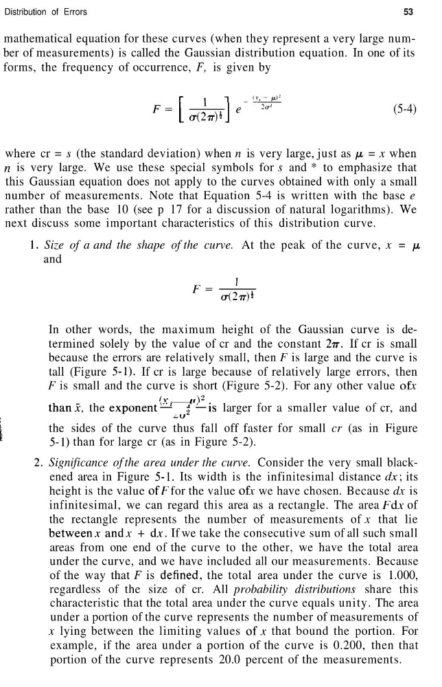
forms, the frequency of occurrence, F, is given by
I CT(27r)*J
(5-4)
where cr = s (the standard deviation) when n is very large, just as pi = x when
H is very large. We use these special symbols for s and * to emphasize that
this Gaussian equation does not apply to the curves obtained with only a small
number of measurements. Note that Equation 5-4 is written with the base e
rather than the base 10 (see p 17 for a discussion of natural logarithms). We
next discuss some important characteristics of this distribution curve.
1. Size of a and the shape of the curve. At the peak of the curve, x = /j.
and
In other words, the maximum height of the Gaussian curve is determined solely by the value of cr and the constant 2ir. If cr is small
because the errors are relatively small, then F is large and the curve is
tall (Figure 5-1). If cr is large because of relatively large errors, then
F is small and the curve is short (Figure 5-2). For any other value of x
( Y .
/ / ) ^
than.*, the exponent—' j —is larger for a smaller value of cr, and
the sides of the curve thus fall off faster for small cr (as in Figure
5-1) than for large cr (as in Figure 5-2).
Significance of the area under the curve. Consider the very small blackened area in Figure 5-1. Its width is the infinitesimal distance dx; its
height is the value of/
7 for the value of x we have chosen. Because dx is
infinitesimal, we can regard this area as a rectangle. The area Fdx of
the rectangle represents the number of measurements of x that lie
between* and* + d*. If we take the consecutive sum of all such small
areas from one end of the curve to the other, we have the total area
under the curve, and we have included all our measurements. Because
of the way that F is denned, the total area under the curve is 1.000,
regardless of the size of cr. All probability distributions share this
characteristic that the total area under the curve equals unity. The area
under a portion of the curve represents the number of measurements of
x lying between the limiting values of* that bound the portion. For
example, if the area under a portion of the curve is 0.200, then that
portion of the curve represents 20.0 percent of the measurements.
53
mathematical equation for these curves (when they represent a very large number of measurements) is called the Gaussian distribution equation. In one of its
forms, the frequency of occurrence, F, is given by
I CT(27r)*J
(5-4)
where cr = s (the standard deviation) when n is very large, just as pi = x when
H is very large. We use these special symbols for s and * to emphasize that
this Gaussian equation does not apply to the curves obtained with only a small
number of measurements. Note that Equation 5-4 is written with the base e
rather than the base 10 (see p 17 for a discussion of natural logarithms). We
next discuss some important characteristics of this distribution curve.
1. Size of a and the shape of the curve. At the peak of the curve, x = /j.
and
In other words, the maximum height of the Gaussian curve is determined solely by the value of cr and the constant 2ir. If cr is small
because the errors are relatively small, then F is large and the curve is
tall (Figure 5-1). If cr is large because of relatively large errors, then
F is small and the curve is short (Figure 5-2). For any other value of x
( Y .
/ / ) ^
than.*, the exponent—' j —is larger for a smaller value of cr, and
the sides of the curve thus fall off faster for small cr (as in Figure
5-1) than for large cr (as in Figure 5-2).
Significance of the area under the curve. Consider the very small blackened area in Figure 5-1. Its width is the infinitesimal distance dx; its
height is the value of/
7 for the value of x we have chosen. Because dx is
infinitesimal, we can regard this area as a rectangle. The area Fdx of
the rectangle represents the number of measurements of x that lie
between* and* + d*. If we take the consecutive sum of all such small
areas from one end of the curve to the other, we have the total area
under the curve, and we have included all our measurements. Because
of the way that F is denned, the total area under the curve is 1.000,
regardless of the size of cr. All probability distributions share this
characteristic that the total area under the curve equals unity. The area
under a portion of the curve represents the number of measurements of
x lying between the limiting values of* that bound the portion. For
example, if the area under a portion of the curve is 0.200, then that
portion of the curve represents 20.0 percent of the measurements.