

of degree n. Then the matrix A satisfies this
particular polynomial equation.
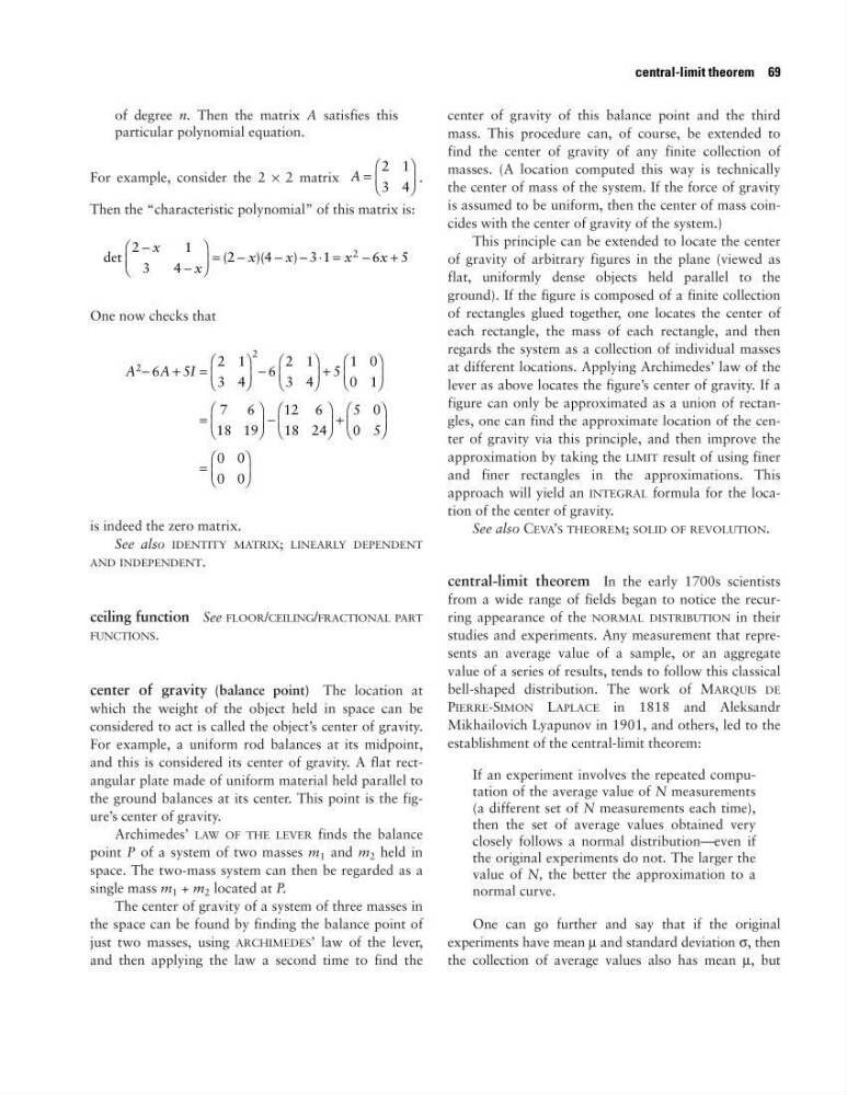
For example, consider the 2 × 2 matrix
.
Then the “characteristic polynomial” of this matrix is:
One now checks that
is indeed the zero matrix.
See also IDENTITY MATRIX; LINEARLY DEPENDENT
AND INDEPENDENT.
ceiling function See FLOOR/CEILING/FRACTIONAL PART
FUNCTIONS.
center of gravity (balance point) The location at
which the weight of the object held in space can be
considered to act is called the object’s center of gravity.
For example, a uniform rod balances at its midpoint,
and this is considered its center of gravity. A flat rectangular plate made of uniform material held parallel to
the ground balances at its center. This point is the figure’s center of gravity.
Archimedes’ LAW OF THE LEVER finds the balance
point P of a system of two masses m 1 and m 2 held in
space. The two-mass system can then be regarded as a
single mass m 1 + m 2 located at P.
The center of gravity of a system of three masses in
the space can be found by finding the balance point of
just two masses, using ARCHIMEDES’ law of the lever,
and then applying the law a second time to find the
center of gravity of this balance point and the third
mass. This procedure can, of course, be extended to
find the center of gravity of any finite collection of
masses. (A location computed this way is technically
the center of mass of the system. If the force of gravity
is assumed to be uniform, then the center of mass coincides with the center of gravity of the system.)
This principle can be extended to locate the center
of gravity of arbitrary figures in the plane (viewed as
flat, uniformly dense objects held parallel to the
ground). If the figure is composed of a finite collection
of rectangles glued together, one locates the center of
each rectangle, the mass of each rectangle, and then
regards the system as a collection of individual masses
at different locations. Applying Archimedes’ law of the
lever as above locates the figure’s center of gravity. If a
figure can only be approximated as a union of rectangles, one can find the approximate location of the center of gravity via this principle, and then improve the
approximation by taking the LIMIT result of using finer
and finer rectangles in the approximations. This
approach will yield an INTEGRAL formula for the location of the center of gravity.
See also CEVA’S THEOREM; SOLID OF REVOLUTION.
central-limit theorem In the early 1700s scientists
from a wide range of fields began to notice the recurring appearance of the NORMAL DISTRIBUTION in their
studies and experiments. Any measurement that represents an average value of a sample, or an aggregate
value of a series of results, tends to follow this classical
bell-shaped distribution. The work of MARQUIS DE
PIERRE-SIMON LAPLACE in 1818 and Aleksandr
Mikhailovich Lyapunov in 1901, and others, led to the
establishment of the central-limit theorem:
If an experiment involves the repeated computation of the average value of N measurements
(a different set of N measurements each time),
then the set of average values obtained very
closely follows a normal distribution—even if
the original experiments do not. The larger the
value of N, the better the approximation to a
normal curve.
One can go further and say that if the original
experiments have mean µ and standard deviation σ, then
the collection of average values also has mean µ, but
A
A I
2
2
6
5
2 1
3 4
6
2 1
3 4
5
1 0
0 1
7 6
18 19
12 6
18 24
5 0
0 5
0 0
0 0
−
+ =
−
+
=
−
+
=
det
(
)(
)
2
1
3
4
2
4
3 1
6
5
2
−
−
= −
− − ⋅ =
−
+
x
x
x
x
x
x
A =
2 1
3 4
central-limit theorem 69
particular polynomial equation.
For example, consider the 2 × 2 matrix
.
Then the “characteristic polynomial” of this matrix is:
One now checks that
is indeed the zero matrix.
See also IDENTITY MATRIX; LINEARLY DEPENDENT
AND INDEPENDENT.
ceiling function See FLOOR/CEILING/FRACTIONAL PART
FUNCTIONS.
center of gravity (balance point) The location at
which the weight of the object held in space can be
considered to act is called the object’s center of gravity.
For example, a uniform rod balances at its midpoint,
and this is considered its center of gravity. A flat rectangular plate made of uniform material held parallel to
the ground balances at its center. This point is the figure’s center of gravity.
Archimedes’ LAW OF THE LEVER finds the balance
point P of a system of two masses m 1 and m 2 held in
space. The two-mass system can then be regarded as a
single mass m 1 + m 2 located at P.
The center of gravity of a system of three masses in
the space can be found by finding the balance point of
just two masses, using ARCHIMEDES’ law of the lever,
and then applying the law a second time to find the
center of gravity of this balance point and the third
mass. This procedure can, of course, be extended to
find the center of gravity of any finite collection of
masses. (A location computed this way is technically
the center of mass of the system. If the force of gravity
is assumed to be uniform, then the center of mass coincides with the center of gravity of the system.)
This principle can be extended to locate the center
of gravity of arbitrary figures in the plane (viewed as
flat, uniformly dense objects held parallel to the
ground). If the figure is composed of a finite collection
of rectangles glued together, one locates the center of
each rectangle, the mass of each rectangle, and then
regards the system as a collection of individual masses
at different locations. Applying Archimedes’ law of the
lever as above locates the figure’s center of gravity. If a
figure can only be approximated as a union of rectangles, one can find the approximate location of the center of gravity via this principle, and then improve the
approximation by taking the LIMIT result of using finer
and finer rectangles in the approximations. This
approach will yield an INTEGRAL formula for the location of the center of gravity.
See also CEVA’S THEOREM; SOLID OF REVOLUTION.
central-limit theorem In the early 1700s scientists
from a wide range of fields began to notice the recurring appearance of the NORMAL DISTRIBUTION in their
studies and experiments. Any measurement that represents an average value of a sample, or an aggregate
value of a series of results, tends to follow this classical
bell-shaped distribution. The work of MARQUIS DE
PIERRE-SIMON LAPLACE in 1818 and Aleksandr
Mikhailovich Lyapunov in 1901, and others, led to the
establishment of the central-limit theorem:
If an experiment involves the repeated computation of the average value of N measurements
(a different set of N measurements each time),
then the set of average values obtained very
closely follows a normal distribution—even if
the original experiments do not. The larger the
value of N, the better the approximation to a
normal curve.
One can go further and say that if the original
experiments have mean µ and standard deviation σ, then
the collection of average values also has mean µ, but
A
A I
2
2
6
5
2 1
3 4
6
2 1
3 4
5
1 0
0 1
7 6
18 19
12 6
18 24
5 0
0 5
0 0
0 0
−
+ =
−
+
=
−
+
=
det
(
)(
)
2
1
3
4
2
4
3 1
6
5
2
−
−
= −
− − ⋅ =
−
+
x
x
x
x
x
x
A =
2 1
3 4
central-limit theorem 69