

summarized by their mean or median, but a set of
data values scattered about a large range of values is
not well represented by a single measure of central
tendency. For example, the two data sets 4.1, 4.1,
4.2, 4.3, 4.4 and 0.1, 0.3, 1.3, 7.8, 11.6 both have
mean 4.22. This provides a good representative
value for the first data set, but not the second.
The usual statistical measures of scatter are
given as follows:
a. The range of a data set is the difference between
the lowest and highest values in the set. For
example, the range of the data set 4, 5, 8, 8 is
8 – 4 = 4.
The range is a very simplistic measure of dispersion and does not reveal any information
about how the data values are distributed. It is
also highly affected by extremely low or high values in the data set. However, the range is often a
useful measurement in practical daily issues. For
example, weather forecasts usually give the range
of temperatures to expect for the day.
b. The deviation of a single data value is the difference between that value and the mean of the data
set, written as a positive quantity. For example, in
the data set 4, 5, 8, 8 with mean 6.25, the deviation of the data value 5 is |5 – 6.25| = 1.25, and
the data value 8 has deviation |8 – 6.25| = 1.75.
The average deviation of all data values gives
a good measure of overall scatter. For example,
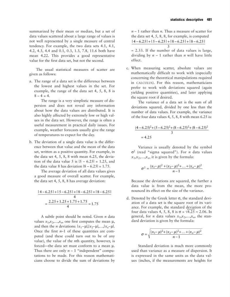
the data set 4, 5, 8, 8 has average deviation:
A subtle point should be noted. Given n data
values x 1 ,x 2 ,…,x n , one first computes the mean µ,
and then the n deviations: |x 1 – µ|,|x 2 – µ|,…,|x n – µ|.
Once the first n–1 of these quantities are computed (and these could turn out to be of any
value), the value of the nth quantity, however, is
forced—the data set must conform to a mean µ.
Thus there are only n – 1 “independent” computations to be made. For this reason mathematicians choose to divide the sum of deviations by
n – 1 rather than n. Thus a measure of scatter for
the data set 4, 5, 8, 8, for example, is computed
≈ 2.33. If the number of data values is large,
dividing by n – 1 rather than n will have little
effect.
c. When measuring scatter, absolute values are
mathematically difficult to work with (especially
concerning the theoretical manipulations required
in CALCULUS). For this reason, mathematicians
prefer to work with deviations squared (again
yielding positive quantities), and later applying
the square root if desired.
The variance of a data set is the sum of all
deviations squared, divided by one less than the
number of data values. For example, the variance
of the four data values 4, 5, 8, 8 with mean 6.25 is:
Variance is usually denoted by the symbol
σ
2 (read “sigma squared”). For n data values
x 1 ,x 2 ,…,x n , it is given by the formula:
Because the deviations are squared, the further a
data value is from the mean, the more pronounced its effect on the size of the variance.
d. Denoted by the Greek letter σ, the standard deviation of a data set is the square root of its variance. For example, the standard deviation of the
four data values 4, 5, 8, 8 is σ = √
–
4.25 ≈ 2.06. In
general, for n data values x 1 ,x 2 ,…,x n , the standard deviation is given by the formula:
Standard deviation is much more commonly
used than variance as a measure of dispersion. It
is expressed in the same units as the data values (inches, if the measurements are heights for
σ
µ
µ
µ
=
−
+
−
+ +
−
−
(
) (
)
(
)
x
x
x
n
n
1
2
2
2
2
1
K
σ
µ
µ
µ
2
1
2
2
2
2
1
=
−
+
−
+ +
−
−
(
) (
)
(
)
x
x
x
n
n
K
(
. ) (
. ) (
. ) (
. )
.
4 6 25
5 6 25
8 6 25
8 6 25
3
4 25
2
2
2
2
−
+ −
+ −
+ −
=
|
. | |
. | |
. | |
. |
4 6 25
5 6 25
8 6 25
8 6 25
3
−
+ −
+ −
+ −
|
. | |
. | |
. | |
. |
.
.
.
.
.
4 6 25
5 6 25
8 6 25
8 6 25
4
2 25 1 25 1 75 1 75
4
1 75
−
+ −
+ −
+ −
=
+
+
+
=
statistics: descriptive 481
data values scattered about a large range of values is
not well represented by a single measure of central
tendency. For example, the two data sets 4.1, 4.1,
4.2, 4.3, 4.4 and 0.1, 0.3, 1.3, 7.8, 11.6 both have
mean 4.22. This provides a good representative
value for the first data set, but not the second.
The usual statistical measures of scatter are
given as follows:
a. The range of a data set is the difference between
the lowest and highest values in the set. For
example, the range of the data set 4, 5, 8, 8 is
8 – 4 = 4.
The range is a very simplistic measure of dispersion and does not reveal any information
about how the data values are distributed. It is
also highly affected by extremely low or high values in the data set. However, the range is often a
useful measurement in practical daily issues. For
example, weather forecasts usually give the range
of temperatures to expect for the day.
b. The deviation of a single data value is the difference between that value and the mean of the data
set, written as a positive quantity. For example, in
the data set 4, 5, 8, 8 with mean 6.25, the deviation of the data value 5 is |5 – 6.25| = 1.25, and
the data value 8 has deviation |8 – 6.25| = 1.75.
The average deviation of all data values gives
a good measure of overall scatter. For example,
the data set 4, 5, 8, 8 has average deviation:
A subtle point should be noted. Given n data
values x 1 ,x 2 ,…,x n , one first computes the mean µ,
and then the n deviations: |x 1 – µ|,|x 2 – µ|,…,|x n – µ|.
Once the first n–1 of these quantities are computed (and these could turn out to be of any
value), the value of the nth quantity, however, is
forced—the data set must conform to a mean µ.
Thus there are only n – 1 “independent” computations to be made. For this reason mathematicians choose to divide the sum of deviations by
n – 1 rather than n. Thus a measure of scatter for
the data set 4, 5, 8, 8, for example, is computed
≈ 2.33. If the number of data values is large,
dividing by n – 1 rather than n will have little
effect.
c. When measuring scatter, absolute values are
mathematically difficult to work with (especially
concerning the theoretical manipulations required
in CALCULUS). For this reason, mathematicians
prefer to work with deviations squared (again
yielding positive quantities), and later applying
the square root if desired.
The variance of a data set is the sum of all
deviations squared, divided by one less than the
number of data values. For example, the variance
of the four data values 4, 5, 8, 8 with mean 6.25 is:
Variance is usually denoted by the symbol
σ
2 (read “sigma squared”). For n data values
x 1 ,x 2 ,…,x n , it is given by the formula:
Because the deviations are squared, the further a
data value is from the mean, the more pronounced its effect on the size of the variance.
d. Denoted by the Greek letter σ, the standard deviation of a data set is the square root of its variance. For example, the standard deviation of the
four data values 4, 5, 8, 8 is σ = √
–
4.25 ≈ 2.06. In
general, for n data values x 1 ,x 2 ,…,x n , the standard deviation is given by the formula:
Standard deviation is much more commonly
used than variance as a measure of dispersion. It
is expressed in the same units as the data values (inches, if the measurements are heights for
σ
µ
µ
µ
=
−
+
−
+ +
−
−
(
) (
)
(
)
x
x
x
n
n
1
2
2
2
2
1
K
σ
µ
µ
µ
2
1
2
2
2
2
1
=
−
+
−
+ +
−
−
(
) (
)
(
)
x
x
x
n
n
K
(
. ) (
. ) (
. ) (
. )
.
4 6 25
5 6 25
8 6 25
8 6 25
3
4 25
2
2
2
2
−
+ −
+ −
+ −
=
|
. | |
. | |
. | |
. |
4 6 25
5 6 25
8 6 25
8 6 25
3
−
+ −
+ −
+ −
|
. | |
. | |
. | |
. |
.
.
.
.
.
4 6 25
5 6 25
8 6 25
8 6 25
4
2 25 1 25 1 75 1 75
4
1 75
−
+ −
+ −
+ −
=
+
+
+
=
statistics: descriptive 481