

the theory of gravitation in the years that followed. He
found applications of this work to the theory of electromagnetism in 1813 and to the theory of heat transfer in 1815.
Late in his career, Poisson’s interests turned toward
probability. Fascinated by studies of societal behavior,
he began to analyze the probability of a random event
occurring within a given interval of time given that its
likelihood of happening is very small, but the number
of opportunities for it to occur is large. This work led
to his discovery of the POISSON DISTRIBUTION, as it is
called today, details of which he published in 1837.
Poisson was a prolific writer and published over
300 mathematical works during his career. Unfortunately, scholars at the time generally did not regard his
latter work important, and Poisson never enjoyed the
full respect of the mathematics community. It was only
after his death, on April 25, 1840, that the significance
of his many innovative ideas became apparent.
Poisson distribution See BINOMIAL DISTRIBUTION.
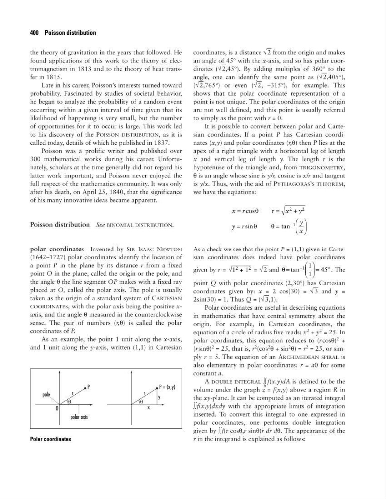
polar coordinates Invented by SIR ISAAC NEWTON
(1642–1727) polar coordinates identify the location of
a point P in the plane by its distance r from a fixed
point O in the plane, called the origin or the pole, and
the angle θ the line segment OP makes with a fixed ray
placed at O, called the polar axis. The pole is usually
taken as the origin of a standard system of CARTESIAN
COORDINATES, with the polar axis being the positive xaxis, and the angle θ measured in the counterclockwise
sense. The pair of numbers (r,θ) is called the polar
coordinates of P.
As an example, the point 1 unit along the x-axis,
and 1 unit along the y-axis, written (1,1) in Cartesian
coordinates, is a distance √
–
2 from the origin and makes
an angle of 45° with the x-axis, and so has polar coordinates (√
–
2,45°). By adding multiples of 360° to the
angle, one can identify the same point as (√
–
2,405°),
(√
–
2,765°) or even (√
–
2, –315°), for example. This
shows that the polar coordinate representation of a
point is not unique. The polar coordinates of the origin
are not well defined, and this point is usually referred
to simply as the point with r = 0.
It is possible to convert between polar and Cartesian coordinates. If a point P has Cartesian coordinates (x,y) and polar coordinates (r,θ) then P lies at the
apex of a right triangle with a horizontal leg of length
x and vertical leg of length y. The length r is the
hypotenuse of the triangle and, from TRIGONOMETRY,
θ is an angle whose sine is y/r, cosine is x/r and tangent
is y/x. Thus, with the aid of PYTHAGORAS’S THEOREM,
we have the equations:
As a check we see that the point P = (1,1) given in Cartesian coordinates does indeed have polar coordinates
given by r =
= √
–
2 and
. The
point Q with polar coordinates (2,30°) has Cartesian
coordinates given by: x = 2 cos(30) = √
–
3 and y =
2sin(30) = 1. Thus Q = (√
–
3,1).
Polar coordinates are useful in describing equations
in mathematics that have central symmetry about the
origin. For example, in Cartesian coordinates, the
equation of a circle of radius five reads: x
2 + y
2 = 25. In
polar coordinates, this equation reduces to (rcosθ)
2 +
(rsinθ)
2 = 25, that is, r
2
(cos
2
θ + sin
2
θ) = r
2 = 25, or simply r = 5. The equation of an ARCHIMEDEAN SPIRAL is
also elementary in polar coordinates: r = aθ for some
constant a.
A DOUBLE INTEGRAL ∫
R
∫ f(x,y)dA is defined to be the
volume under the graph z = f(x,y) above a region R in
the xy-plane. It can be computed as an iterated integral
∫∫f(x,y)dxdy with the appropriate limits of integration
inserted. To convert this integral to one expressed in
polar coordinates, one performs double integration
given by ∫∫f(r cosθ,r sinθ)r dr dθ. The appearance of the
r in the integrand is explained as follows:
θ =
= °
−
tan
1 1
1
45
√1
2 + 1
2
x r
r
x y
y r
y
x
=
=
+
=
=
−
cos
sin
tan
θ
θ
θ
2
2
1
400 Poisson distribution
Polar coordinates
found applications of this work to the theory of electromagnetism in 1813 and to the theory of heat transfer in 1815.
Late in his career, Poisson’s interests turned toward
probability. Fascinated by studies of societal behavior,
he began to analyze the probability of a random event
occurring within a given interval of time given that its
likelihood of happening is very small, but the number
of opportunities for it to occur is large. This work led
to his discovery of the POISSON DISTRIBUTION, as it is
called today, details of which he published in 1837.
Poisson was a prolific writer and published over
300 mathematical works during his career. Unfortunately, scholars at the time generally did not regard his
latter work important, and Poisson never enjoyed the
full respect of the mathematics community. It was only
after his death, on April 25, 1840, that the significance
of his many innovative ideas became apparent.
Poisson distribution See BINOMIAL DISTRIBUTION.
polar coordinates Invented by SIR ISAAC NEWTON
(1642–1727) polar coordinates identify the location of
a point P in the plane by its distance r from a fixed
point O in the plane, called the origin or the pole, and
the angle θ the line segment OP makes with a fixed ray
placed at O, called the polar axis. The pole is usually
taken as the origin of a standard system of CARTESIAN
COORDINATES, with the polar axis being the positive xaxis, and the angle θ measured in the counterclockwise
sense. The pair of numbers (r,θ) is called the polar
coordinates of P.
As an example, the point 1 unit along the x-axis,
and 1 unit along the y-axis, written (1,1) in Cartesian
coordinates, is a distance √
–
2 from the origin and makes
an angle of 45° with the x-axis, and so has polar coordinates (√
–
2,45°). By adding multiples of 360° to the
angle, one can identify the same point as (√
–
2,405°),
(√
–
2,765°) or even (√
–
2, –315°), for example. This
shows that the polar coordinate representation of a
point is not unique. The polar coordinates of the origin
are not well defined, and this point is usually referred
to simply as the point with r = 0.
It is possible to convert between polar and Cartesian coordinates. If a point P has Cartesian coordinates (x,y) and polar coordinates (r,θ) then P lies at the
apex of a right triangle with a horizontal leg of length
x and vertical leg of length y. The length r is the
hypotenuse of the triangle and, from TRIGONOMETRY,
θ is an angle whose sine is y/r, cosine is x/r and tangent
is y/x. Thus, with the aid of PYTHAGORAS’S THEOREM,
we have the equations:
As a check we see that the point P = (1,1) given in Cartesian coordinates does indeed have polar coordinates
given by r =
= √
–
2 and
. The
point Q with polar coordinates (2,30°) has Cartesian
coordinates given by: x = 2 cos(30) = √
–
3 and y =
2sin(30) = 1. Thus Q = (√
–
3,1).
Polar coordinates are useful in describing equations
in mathematics that have central symmetry about the
origin. For example, in Cartesian coordinates, the
equation of a circle of radius five reads: x
2 + y
2 = 25. In
polar coordinates, this equation reduces to (rcosθ)
2 +
(rsinθ)
2 = 25, that is, r
2
(cos
2
θ + sin
2
θ) = r
2 = 25, or simply r = 5. The equation of an ARCHIMEDEAN SPIRAL is
also elementary in polar coordinates: r = aθ for some
constant a.
A DOUBLE INTEGRAL ∫
R
∫ f(x,y)dA is defined to be the
volume under the graph z = f(x,y) above a region R in
the xy-plane. It can be computed as an iterated integral
∫∫f(x,y)dxdy with the appropriate limits of integration
inserted. To convert this integral to one expressed in
polar coordinates, one performs double integration
given by ∫∫f(r cosθ,r sinθ)r dr dθ. The appearance of the
r in the integrand is explained as follows:
θ =
= °
−
tan
1 1
1
45
√1
2 + 1
2
x r
r
x y
y r
y
x
=
=
+
=
=
−
cos
sin
tan
θ
θ
θ
2
2
1
400 Poisson distribution
Polar coordinates