

linear programming The branch of mathematics
concerned with finding the maximum or minimum values of linear functions, that is, functions involving variables raised only to the first power, subject to a number
of inequalities that must remain true, is called linear
programming. This field has profound applications to
economics and industry and is an area of active
research. While, in principle, OPTIMIZATION problems
of this type are straightforward to solve, practical
problems may involve well over 100 variables and be
difficult to analyze. The challenge is to find efficient
techniques for finding solutions.
The principle of linear programming is best illustrated with an example. Suppose, for instance, we wish
to find the maximum value of the function U = 4x – 3y
subject to the constraints x ≥ 0, y ≥ 0, x ≤ 1, and y ≤ 1.
In this example, the constraints define a unit square in
the plane, and we wish to find the point (x, y) in this
“feasible region” that provides the largest value for the
“objective function”U = 4x – 3y.
Reasoning backward, note that each possible value
c of the objective function defines a line 4x – 3y = c of
slope 4/3. As the value of c varies, this line sweeps
across the plane. Starting with a large value of c and
decreasing its value, we thus seek the first value, of c
that produces a line that touches the feasibility region.
Clearly, this will occur at one of the vertices of the
square. Checking all four vertices, (0,0), (1,0), (0,1),
and (1,1), we see that x = 1, y = 0 gives the largest possible value 4 for U.
In general, the constraint conditions define a polygonal region in space, and the maximal and minimal
values of U can only occur at vertices of the region.
Linear programming then seeks to find efficient methods for checking which vertices yield the largest and
smallest values for U.
See also OPERATIONS RESEARCH.
linear transformation A map T : V → W between
two VECTOR SPACEs V and W is called a linear transformation if the following two conditions hold:
i. T(a + b) = T(a) + T(b) for any two vectors a and b
ii. T(ka) = kT(a) for any number k and any vector a
If the vector spaces V and W represent the set of all
points in the plane or in three-dimensional space, then
a linear transformation is an example of a GEOMETRIC
TRANSFORMATION that takes straight lines to straight
lines. For instance, rotations and reflections are linear
transformations. However, not every geometric transformation is a linear transformation. Although a translation, for example, preserves straight lines in the
plane, it does not satisfy the first condition described
above and so is not a linear transformation.
If e 1 e 2 ,…,e n is a basis for the vector space V, then
any vector a in V can be written as a linear combination of these basis vectors:
a = c 1 e 1 + c 2 e 2 +…+ c n e n
for some numbers c 1 , c 2 ,…, c n . Thus the value of the
linear transformation T is completely determined by its
values on the basis vectors:
T(a) = T(c 1 e 1 + c 2 e 2 +…+ c n e n )
= c 1 T(e 1 ) + c 2 T(e 2 ) +…+ c n T(e n )
If f 1 ,f 2 ,…,f m is a basis for the second vector space W,
then each vector T(e j ) is a linear combination of these
basis vectors:
T(e j ) = a 1j f 1 + a 2j f 2 +…+ a mj f m
Thus the numbers a ij completely specify how the linear transformation works. Let A be the MATRIX with
(i,j)th entry equal to a ij . This shows that every linear
transformation is represented by a matrix. Moreover,
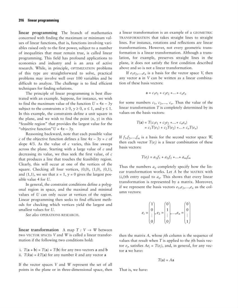
if we represent the basis vectors e 1 ,e 2 ,…,e n as the column vectors:
then the matrix A, whose jth column is the sequence of
values that result when T is applied to the jth basis vector e j , satisfies Ae j = T(e j ), and, in general, for any vector a we have:
T(a) = Aa
That is, we have:
e
e
e
i
n
=
=
=
1
0
0
0
1
0
0
0
1
2
M
M
K
M
,
, ,
316 linear programming
concerned with finding the maximum or minimum values of linear functions, that is, functions involving variables raised only to the first power, subject to a number
of inequalities that must remain true, is called linear
programming. This field has profound applications to
economics and industry and is an area of active
research. While, in principle, OPTIMIZATION problems
of this type are straightforward to solve, practical
problems may involve well over 100 variables and be
difficult to analyze. The challenge is to find efficient
techniques for finding solutions.
The principle of linear programming is best illustrated with an example. Suppose, for instance, we wish
to find the maximum value of the function U = 4x – 3y
subject to the constraints x ≥ 0, y ≥ 0, x ≤ 1, and y ≤ 1.
In this example, the constraints define a unit square in
the plane, and we wish to find the point (x, y) in this
“feasible region” that provides the largest value for the
“objective function”U = 4x – 3y.
Reasoning backward, note that each possible value
c of the objective function defines a line 4x – 3y = c of
slope 4/3. As the value of c varies, this line sweeps
across the plane. Starting with a large value of c and
decreasing its value, we thus seek the first value, of c
that produces a line that touches the feasibility region.
Clearly, this will occur at one of the vertices of the
square. Checking all four vertices, (0,0), (1,0), (0,1),
and (1,1), we see that x = 1, y = 0 gives the largest possible value 4 for U.
In general, the constraint conditions define a polygonal region in space, and the maximal and minimal
values of U can only occur at vertices of the region.
Linear programming then seeks to find efficient methods for checking which vertices yield the largest and
smallest values for U.
See also OPERATIONS RESEARCH.
linear transformation A map T : V → W between
two VECTOR SPACEs V and W is called a linear transformation if the following two conditions hold:
i. T(a + b) = T(a) + T(b) for any two vectors a and b
ii. T(ka) = kT(a) for any number k and any vector a
If the vector spaces V and W represent the set of all
points in the plane or in three-dimensional space, then
a linear transformation is an example of a GEOMETRIC
TRANSFORMATION that takes straight lines to straight
lines. For instance, rotations and reflections are linear
transformations. However, not every geometric transformation is a linear transformation. Although a translation, for example, preserves straight lines in the
plane, it does not satisfy the first condition described
above and so is not a linear transformation.
If e 1 e 2 ,…,e n is a basis for the vector space V, then
any vector a in V can be written as a linear combination of these basis vectors:
a = c 1 e 1 + c 2 e 2 +…+ c n e n
for some numbers c 1 , c 2 ,…, c n . Thus the value of the
linear transformation T is completely determined by its
values on the basis vectors:
T(a) = T(c 1 e 1 + c 2 e 2 +…+ c n e n )
= c 1 T(e 1 ) + c 2 T(e 2 ) +…+ c n T(e n )
If f 1 ,f 2 ,…,f m is a basis for the second vector space W,
then each vector T(e j ) is a linear combination of these
basis vectors:
T(e j ) = a 1j f 1 + a 2j f 2 +…+ a mj f m
Thus the numbers a ij completely specify how the linear transformation works. Let A be the MATRIX with
(i,j)th entry equal to a ij . This shows that every linear
transformation is represented by a matrix. Moreover,
if we represent the basis vectors e 1 ,e 2 ,…,e n as the column vectors:
then the matrix A, whose jth column is the sequence of
values that result when T is applied to the jth basis vector e j , satisfies Ae j = T(e j ), and, in general, for any vector a we have:
T(a) = Aa
That is, we have:
e
e
e
i
n
=
=
=
1
0
0
0
1
0
0
0
1
2
M
M
K
M
,
, ,
316 linear programming