

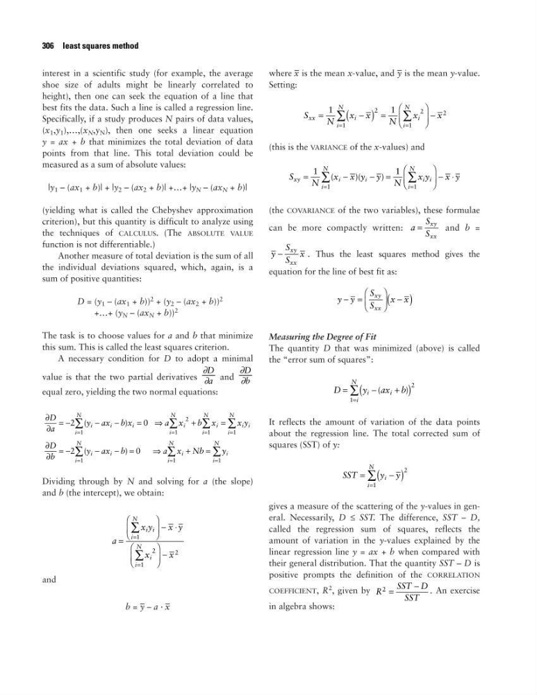
interest in a scientific study (for example, the average
shoe size of adults might be linearly correlated to
height), then one can seek the equation of a line that
best fits the data. Such a line is called a regression line.
Specifically, if a study produces N pairs of data values,
(x 1 ,y 1 ),…,(x N ,y N ), then one seeks a linear equation
y = ax + b that minimizes the total deviation of data
points from that line. This total deviation could be
measured as a sum of absolute values:
|y 1 – (ax 1 + b)| + |y 2 – (ax 2 + b)| +…+ |y N – (ax N + b)|
(yielding what is called the Chebyshev approximation
criterion), but this quantity is difficult to analyze using
the techniques of CALCULUS. (The ABSOLUTE VALUE
function is not differentiable.)
Another measure of total deviation is the sum of all
the individual deviations squared, which, again, is a
sum of positive quantities:
D = (y 1 – (ax 1 + b))
2 + (y 2 – (ax 2 + b))
2
+…+ (y N – (ax N + b))
2
The task is to choose values for a and b that minimize
this sum. This is called the least squares criterion.
A necessary condition for D to adopt a minimal
value is that the two partial derivatives
and
equal zero, yielding the two normal equations:
Dividing through by N and solving for a (the slope)
and b (the intercept), we obtain:
and
b = – y – a · –
x
where –
x is the mean x-value, and – y is the mean y-value.
Setting:
(this is the VARIANCE of the x-values) and
(the COVARIANCE of the two variables), these formulae
can be more compactly written:
and b =
. Thus the least squares method gives the
equation for the line of best fit as:
Measuring the Degree of Fit
The quantity D that was minimized (above) is called
the “error sum of squares”:
It reflects the amount of variation of the data points
about the regression line. The total corrected sum of
squares (SST) of y:
gives a measure of the scattering of the y-values in general. Necessarily, D ≤ SST. The difference, SST – D,
called the regression sum of squares, reflects the
amount of variation in the y-values explained by the
linear regression line y = ax + b when compared with
their general distribution. That the quantity SST – D is
positive prompts the definition of the CORRELATION
COEFFICIENT, R
2
, given by
. An exercise
in algebra shows:
R
SST D
SST
2
=
−
SST
y y
i
i
N
=
−
(
)
=
∑
2
1
D
y
ax b
i
i
i
N
=
−
+
(
)
=
∑
(
)
2
1
y y
S
S
x x
xy
xx
− =
−
( )
y
S
S
x
xy
xx
−
a
S
S
xy
xx
=
S
N
x x y y
N
x y
x y
xy
i
i
i
N
i i
i
N
=
−
− =
− ⋅
=
=
∑
∑
1
1
1
1
(
)(
)
S
N
x x
N
x
x
xx
i
i
N
i
i
N
=
−
(
) =
−
=
=
∑
∑
1
1
2
1
2
1
2
a
x y
x y
x
x
i i
i
N
i
i
N
=
− ⋅
−
=
=
∑
∑
1
2
1
2
∂
∂
= −
−
−
=
⇒
+
=
∂
∂
= −
−
− =
⇒
+
=
=
=
=
=
=
=
=
∑
∑ ∑
∑
∑
∑
∑
D
a
y ax b x
a x
b x
x y
D
b
y ax b
a x Nb
y
i
i
i
i
N
i
i
i
N
i i
i
N
i
N
i
i
i
N
i
i
N
i
i
N
2
0
2
0
1
2
1
1
1
1
1
1
(
)
(
)
∂D
––
∂b
∂D
––
∂a
306 least squares method
shoe size of adults might be linearly correlated to
height), then one can seek the equation of a line that
best fits the data. Such a line is called a regression line.
Specifically, if a study produces N pairs of data values,
(x 1 ,y 1 ),…,(x N ,y N ), then one seeks a linear equation
y = ax + b that minimizes the total deviation of data
points from that line. This total deviation could be
measured as a sum of absolute values:
|y 1 – (ax 1 + b)| + |y 2 – (ax 2 + b)| +…+ |y N – (ax N + b)|
(yielding what is called the Chebyshev approximation
criterion), but this quantity is difficult to analyze using
the techniques of CALCULUS. (The ABSOLUTE VALUE
function is not differentiable.)
Another measure of total deviation is the sum of all
the individual deviations squared, which, again, is a
sum of positive quantities:
D = (y 1 – (ax 1 + b))
2 + (y 2 – (ax 2 + b))
2
+…+ (y N – (ax N + b))
2
The task is to choose values for a and b that minimize
this sum. This is called the least squares criterion.
A necessary condition for D to adopt a minimal
value is that the two partial derivatives
and
equal zero, yielding the two normal equations:
Dividing through by N and solving for a (the slope)
and b (the intercept), we obtain:
and
b = – y – a · –
x
where –
x is the mean x-value, and – y is the mean y-value.
Setting:
(this is the VARIANCE of the x-values) and
(the COVARIANCE of the two variables), these formulae
can be more compactly written:
and b =
. Thus the least squares method gives the
equation for the line of best fit as:
Measuring the Degree of Fit
The quantity D that was minimized (above) is called
the “error sum of squares”:
It reflects the amount of variation of the data points
about the regression line. The total corrected sum of
squares (SST) of y:
gives a measure of the scattering of the y-values in general. Necessarily, D ≤ SST. The difference, SST – D,
called the regression sum of squares, reflects the
amount of variation in the y-values explained by the
linear regression line y = ax + b when compared with
their general distribution. That the quantity SST – D is
positive prompts the definition of the CORRELATION
COEFFICIENT, R
2
, given by
. An exercise
in algebra shows:
R
SST D
SST
2
=
−
SST
y y
i
i
N
=
−
(
)
=
∑
2
1
D
y
ax b
i
i
i
N
=
−
+
(
)
=
∑
(
)
2
1
y y
S
S
x x
xy
xx
− =
−
( )
y
S
S
x
xy
xx
−
a
S
S
xy
xx
=
S
N
x x y y
N
x y
x y
xy
i
i
i
N
i i
i
N
=
−
− =
− ⋅
=
=
∑
∑
1
1
1
1
(
)(
)
S
N
x x
N
x
x
xx
i
i
N
i
i
N
=
−
(
) =
−
=
=
∑
∑
1
1
2
1
2
1
2
a
x y
x y
x
x
i i
i
N
i
i
N
=
− ⋅
−
=
=
∑
∑
1
2
1
2
∂
∂
= −
−
−
=
⇒
+
=
∂
∂
= −
−
− =
⇒
+
=
=
=
=
=
=
=
=
∑
∑ ∑
∑
∑
∑
∑
D
a
y ax b x
a x
b x
x y
D
b
y ax b
a x Nb
y
i
i
i
i
N
i
i
i
N
i i
i
N
i
N
i
i
i
N
i
i
N
i
i
N
2
0
2
0
1
2
1
1
1
1
1
1
(
)
(
)
∂D
––
∂b
∂D
––
∂a
306 least squares method