

If the sum of payments to all players is zero, then the
game is called a zero-sum game. This means that any
player’s win must be balanced by a loss for some
other players.
The simplest type of game is a two-player zero-sum
game. The choice of actions and the possible results of
the game can be summarized in a “payoff matrix” A, in
which the rows represent the possible actions one
player, player R, can take; the columns the possible
actions of the second player, player C; and the (i,j)-th
entry of the matrix A ij represents the amount player C
must pay to player R if R selects row i and C selects
column j in the play of the game. (If A ij is negative,
then player R pays C a certain amount.) For example,
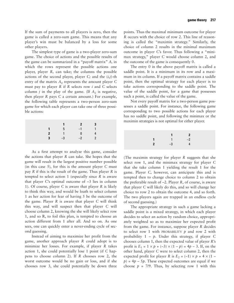
the following table represents a two-person zero-sum
game for which each player can take one of three possible actions:
As a first attempt to analyze this game, consider
the actions that player R can take. She hopes that the
game will result in the largest positive number possible
(in this case 5), for this is the amount player C must
pay R if this is the result of the game. Thus player R is
tempted to select action 1 (especially since R is aware
that player C’s optimal outcome of –3 lies in column
1). Of course, player C is aware that player R is likely
to think this way, and would be loath to select column
1 as her action for fear of having 5 be the outcome of
the game. Player R is aware that player C will think
this way, and will suspect then that player C will
choose column 2, knowing the she will likely select row
1, and so R, to foil this plan, is tempted to choose an
action different from 1 after all. And so on. As one
sees, one can quickly enter a never-ending cycle of second guessing.
Instead of aiming to maximize her profit from the
game, another approach player R could adopt is to
minimize her losses. For example, if player R takes
action 1, she could potentially lose 1 point (if C happens to choose column 2). If R chooses row 2, the
worst outcome would be no gain or loss, and if she
chooses row 3, she could potentially be down three
points. Thus the maximal minimum outcome for player
R occurs with the choice of row 2. This line of reasoning is called the “maximin strategy.” Similarly, the
choice of column 2 results in the minimal maximum
outcome in player C’s favor. Thus following a “minimax strategy,” player C would choose column 2, and
the outcome of the game is consequently 0.
The entry 0 in the above payoff matrix is called a
saddle point. It is a minimum in its row and a maximum in its column. If a payoff matrix contains a saddle
point, then the optimal strategy for each player is to
take actions corresponding to the saddle point. The
value of the saddle point, for a game that possesses
such a point, is called the value of the game.
Not every payoff matrix for a two-person game possesses a saddle point. For instance, the following game
corresponding to two possible actions for each player
has no saddle point, and following the minimax or the
maximin strategies is not optimal for either player.
(The maximin strategy for player R suggests that she
select row 1, and the minimax strategy for player C
that she take column 1 yielding the result 1 for the
game. Player C, however, can anticipate this and is
tempted then to change choice to column 2 to obtain
the preferable result of –2. Player R, of course, is aware
that player C will likely do this, and so will change her
choice to row 2 to obtain the outcome 4, and so forth.
The two players again are trapped in an endless cycle
of second guessing.)
The appropriate strategy in such a game lacking a
saddle point is a mixed strategy, in which each player
decides to select an action by random choice, appropriately weighted so as to maximize her expected profit
from the game. For instance, suppose player R decides
to select row 1 with PROBABILITY p and row 2 with
probability 1 – p. Under this strategy, if player C
chooses column 1, then the expected value of player R’s
profit is E 1 = 1 × p + (–3) × (1 – p) = 4p – 3. If, on the
other hand, player C were to select column 2, then the
expected profit for player R is E 2 = (–1) × p + 4 × (1 –
p) = 4p – 5p. These expected outcomes are equal if we
choose p = 7/9. Thus, by selecting row 1 with this
1
2
1
1
– 2
2
–3
4
1
2
3
1
5
– 1
1
2
1
0
4
3
–3
–2
2
game theory 217
game is called a zero-sum game. This means that any
player’s win must be balanced by a loss for some
other players.
The simplest type of game is a two-player zero-sum
game. The choice of actions and the possible results of
the game can be summarized in a “payoff matrix” A, in
which the rows represent the possible actions one
player, player R, can take; the columns the possible
actions of the second player, player C; and the (i,j)-th
entry of the matrix A ij represents the amount player C
must pay to player R if R selects row i and C selects
column j in the play of the game. (If A ij is negative,
then player R pays C a certain amount.) For example,
the following table represents a two-person zero-sum
game for which each player can take one of three possible actions:
As a first attempt to analyze this game, consider
the actions that player R can take. She hopes that the
game will result in the largest positive number possible
(in this case 5), for this is the amount player C must
pay R if this is the result of the game. Thus player R is
tempted to select action 1 (especially since R is aware
that player C’s optimal outcome of –3 lies in column
1). Of course, player C is aware that player R is likely
to think this way, and would be loath to select column
1 as her action for fear of having 5 be the outcome of
the game. Player R is aware that player C will think
this way, and will suspect then that player C will
choose column 2, knowing the she will likely select row
1, and so R, to foil this plan, is tempted to choose an
action different from 1 after all. And so on. As one
sees, one can quickly enter a never-ending cycle of second guessing.
Instead of aiming to maximize her profit from the
game, another approach player R could adopt is to
minimize her losses. For example, if player R takes
action 1, she could potentially lose 1 point (if C happens to choose column 2). If R chooses row 2, the
worst outcome would be no gain or loss, and if she
chooses row 3, she could potentially be down three
points. Thus the maximal minimum outcome for player
R occurs with the choice of row 2. This line of reasoning is called the “maximin strategy.” Similarly, the
choice of column 2 results in the minimal maximum
outcome in player C’s favor. Thus following a “minimax strategy,” player C would choose column 2, and
the outcome of the game is consequently 0.
The entry 0 in the above payoff matrix is called a
saddle point. It is a minimum in its row and a maximum in its column. If a payoff matrix contains a saddle
point, then the optimal strategy for each player is to
take actions corresponding to the saddle point. The
value of the saddle point, for a game that possesses
such a point, is called the value of the game.
Not every payoff matrix for a two-person game possesses a saddle point. For instance, the following game
corresponding to two possible actions for each player
has no saddle point, and following the minimax or the
maximin strategies is not optimal for either player.
(The maximin strategy for player R suggests that she
select row 1, and the minimax strategy for player C
that she take column 1 yielding the result 1 for the
game. Player C, however, can anticipate this and is
tempted then to change choice to column 2 to obtain
the preferable result of –2. Player R, of course, is aware
that player C will likely do this, and so will change her
choice to row 2 to obtain the outcome 4, and so forth.
The two players again are trapped in an endless cycle
of second guessing.)
The appropriate strategy in such a game lacking a
saddle point is a mixed strategy, in which each player
decides to select an action by random choice, appropriately weighted so as to maximize her expected profit
from the game. For instance, suppose player R decides
to select row 1 with PROBABILITY p and row 2 with
probability 1 – p. Under this strategy, if player C
chooses column 1, then the expected value of player R’s
profit is E 1 = 1 × p + (–3) × (1 – p) = 4p – 3. If, on the
other hand, player C were to select column 2, then the
expected profit for player R is E 2 = (–1) × p + 4 × (1 –
p) = 4p – 5p. These expected outcomes are equal if we
choose p = 7/9. Thus, by selecting row 1 with this
1
2
1
1
– 2
2
–3
4
1
2
3
1
5
– 1
1
2
1
0
4
3
–3
–2
2
game theory 217