

A represents 10, B represents 11, and so forth, with F
representing 15. Each decimal place is a power of a
sixteenth.) Unfortunately no analogous technique is
currently known to compute the ordinary base-10 digits of π with ease.
extrapolation The process of estimating the value
of a function outside a known range of values is called
extrapolation. For example, if the temperature of a
cup of tea was initially 200°F and then was measured
to be 100°F and 50°F 10 and 20 minutes later, respectively, then one might guess that its temperature after
30 minutes would be 25°F. Methods of extrapolation
are normally far less reliable than INTERPOLATION, the
process of estimating function values between known
values. Scientists generally prefer to avoid making predictions based on extrapolation. Meteorologists, however, must use extrapolation techniques to make
weather predictions. Long-range forecasts are generally considered unreliable.
See also POPULATION MODELS.
extreme-value theorem This theorem asserts that a
CONTINUOUS FUNCTION f(x), defined on a closed
INTERVAL [a,b], reaches a maximum value and a minimum value somewhere within that interval. That is,
there is a point c in the interval [a,b] such that f(x),
≤ f(c), for all x in [a,b], and there is another point d in
[a,b] such that f(x) ≥ f(d) for all x in [a,b]. For example, the extreme-value theorem tells us that, on the
interval [1,5] say, the function f(x) = 3x · cos(x
2 + sinx)
does indeed adopt a largest value. It does not tell us,
however, where that maximum value occurs. A point at
which a function has a maximum or minimum value is
called an extremum.
The theorem is intuitively clear if we think of a
continuous function on a closed interval as one whose
graph consists of a single continuous piece with no
gaps, jumps, or holes: in moving a pencil from the left
end point (a,f(a)) to the right end point (b,f(b)), one
would not doubt that there must be a high point on
the curve where f(x) reaches its maximum value, and
a low point where it attains its minimum value. A rigorous proof of the theorem, however, relies on the
notion of the completeness of the real numbers (meaning that no points are missing from the real line). This
is a subtle property, one that was not properly understood until the late 1800s with the invention of a
DEDEKIND CUT. For example, the function f(x) = 2x –
x
2 = x(2 – x) has no maximum value on the interval
[0, 2] if the value 1 is excluded from our considerations. Although this seems an artificial example, one
still needs to be sure that this type of problem can
never occur.
It is vital that the function under consideration be
continuous and that the interval under study be closed
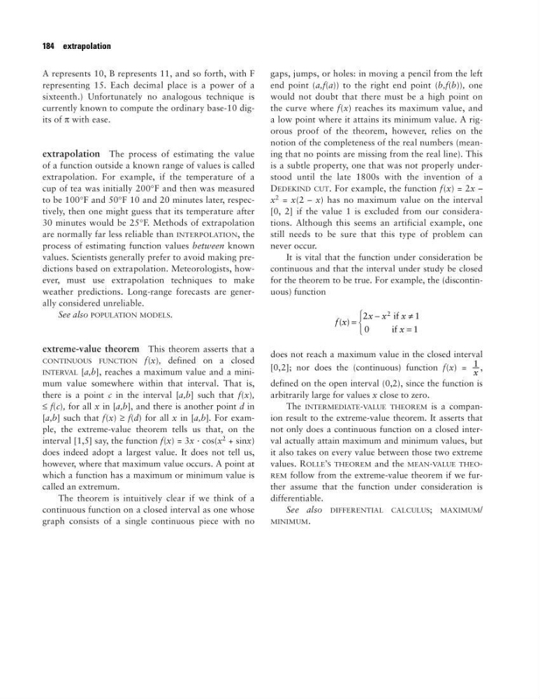
for the theorem to be true. For example, the (discontinuous) function
does not reach a maximum value in the closed interval
[0,2]; nor does the (continuous) function f(x) =
,
defined on the open interval (0,2), since the function is
arbitrarily large for values x close to zero.
The INTERMEDIATE-VALUE THEOREM is a companion result to the extreme-value theorem. It asserts that
not only does a continuous function on a closed interval actually attain maximum and minimum values, but
it also takes on every value between those two extreme
values. ROLLE’S THEOREM and the MEAN-VALUE THEOREM follow from the extreme-value theorem if we further assume that the function under consideration is
differentiable.
See also DIFFERENTIAL CALCULUS; MAXIMUM/
MINIMUM.
1
–
x
f x
x x
x
x
( ) =
−
≠
=
2
1
0
1
2 if
if
184 extrapolation
representing 15. Each decimal place is a power of a
sixteenth.) Unfortunately no analogous technique is
currently known to compute the ordinary base-10 digits of π with ease.
extrapolation The process of estimating the value
of a function outside a known range of values is called
extrapolation. For example, if the temperature of a
cup of tea was initially 200°F and then was measured
to be 100°F and 50°F 10 and 20 minutes later, respectively, then one might guess that its temperature after
30 minutes would be 25°F. Methods of extrapolation
are normally far less reliable than INTERPOLATION, the
process of estimating function values between known
values. Scientists generally prefer to avoid making predictions based on extrapolation. Meteorologists, however, must use extrapolation techniques to make
weather predictions. Long-range forecasts are generally considered unreliable.
See also POPULATION MODELS.
extreme-value theorem This theorem asserts that a
CONTINUOUS FUNCTION f(x), defined on a closed
INTERVAL [a,b], reaches a maximum value and a minimum value somewhere within that interval. That is,
there is a point c in the interval [a,b] such that f(x),
≤ f(c), for all x in [a,b], and there is another point d in
[a,b] such that f(x) ≥ f(d) for all x in [a,b]. For example, the extreme-value theorem tells us that, on the
interval [1,5] say, the function f(x) = 3x · cos(x
2 + sinx)
does indeed adopt a largest value. It does not tell us,
however, where that maximum value occurs. A point at
which a function has a maximum or minimum value is
called an extremum.
The theorem is intuitively clear if we think of a
continuous function on a closed interval as one whose
graph consists of a single continuous piece with no
gaps, jumps, or holes: in moving a pencil from the left
end point (a,f(a)) to the right end point (b,f(b)), one
would not doubt that there must be a high point on
the curve where f(x) reaches its maximum value, and
a low point where it attains its minimum value. A rigorous proof of the theorem, however, relies on the
notion of the completeness of the real numbers (meaning that no points are missing from the real line). This
is a subtle property, one that was not properly understood until the late 1800s with the invention of a
DEDEKIND CUT. For example, the function f(x) = 2x –
x
2 = x(2 – x) has no maximum value on the interval
[0, 2] if the value 1 is excluded from our considerations. Although this seems an artificial example, one
still needs to be sure that this type of problem can
never occur.
It is vital that the function under consideration be
continuous and that the interval under study be closed
for the theorem to be true. For example, the (discontinuous) function
does not reach a maximum value in the closed interval
[0,2]; nor does the (continuous) function f(x) =
,
defined on the open interval (0,2), since the function is
arbitrarily large for values x close to zero.
The INTERMEDIATE-VALUE THEOREM is a companion result to the extreme-value theorem. It asserts that
not only does a continuous function on a closed interval actually attain maximum and minimum values, but
it also takes on every value between those two extreme
values. ROLLE’S THEOREM and the MEAN-VALUE THEOREM follow from the extreme-value theorem if we further assume that the function under consideration is
differentiable.
See also DIFFERENTIAL CALCULUS; MAXIMUM/
MINIMUM.
1
–
x
f x
x x
x
x
( ) =
−
≠
=
2
1
0
1
2 if
if
184 extrapolation