

184
Reach represents the continuity between points of adjacent data. At a greater distance from the intersection of the threshold and the variogram curve, one can no
longer speak of continuity between points. (4) “Distance” is the distance on the
x-axis at which the data in the variogram direction are compared. Each distance
makes one class. This value is often assigned a certain tolerance (offset) in order to
increase the number of input data. Thus, we add a certain value of the offset to the
class boundary, so the variogram classes are represented by certain intervals (e.g.
0.5–1.5, 1.5–2.5, etc.). Usually the offset is set to 1/2 distance values, which maximizes the number of pairs and at the same time the reliability of the spatial analysis
(Wellmer 1998).
6.6.2.2 Kriging
Namely, the kriging method is based on the use of known values of so-called
variable control points, the influence of which on the assessment is expressed by
appropriate weighting coefficients (Wellmer 1998; de Smith et al. 2009). The most
demanding procedure in kriging is to determine the weighting coefficients for each
control point individually. During the assessment, it is necessary to meet certain
criteria, i.e. to be impartial and defined so that the variance of the difference between
the actual and estimated values at the selected points is the smallest (Zeigler et al.
2000). Due to reliable estimates of spatially distributed variables, the kriging method
has found great application in many branches of research. It was primarily created
for the needs of mobile environments and surfaces in mining and geology, for example, as a means of improving the assessment of ore reserves and natural resources.
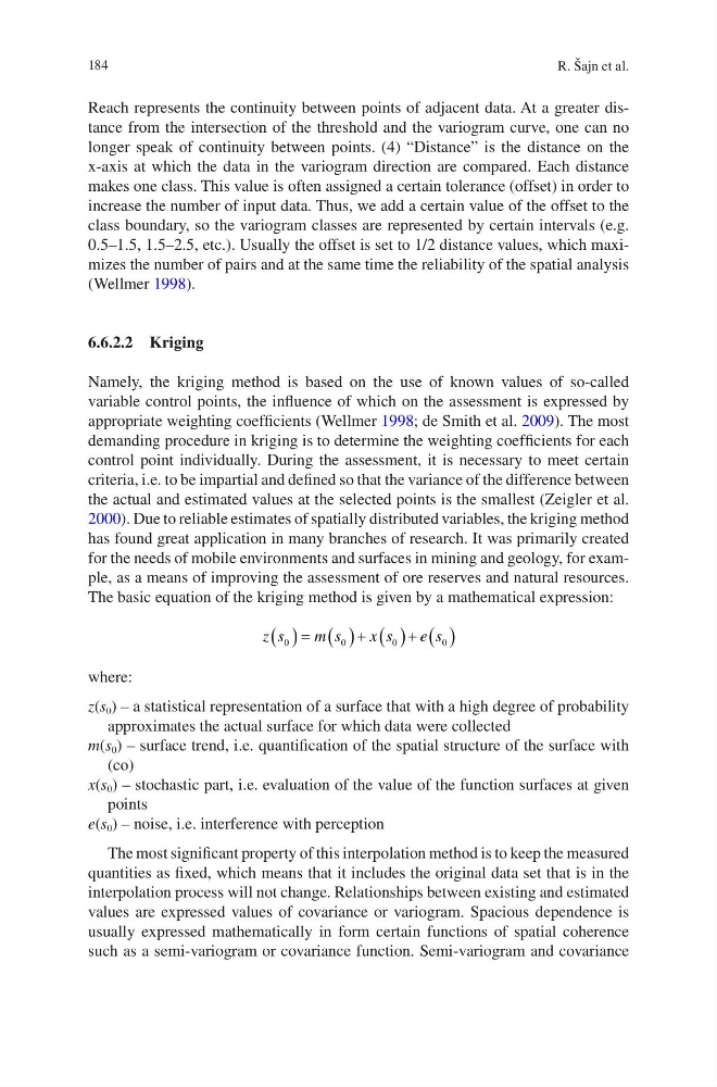
The basic equation of the kriging method is given by a mathematical expression:
z s
m s
x s
e s
0
0
0
0
where:
z(s 0 ) – a statistical representation of a surface that with a high degree of probability
approximates the actual surface for which data were collected
m(s 0 ) – surface trend, i.e. quantification of the spatial structure of the surface with
(co)
x(s 0 ) – stochastic part, i.e. evaluation of the value of the function surfaces at given
points
e(s 0 ) – noise, i.e. interference with perception
The most significant property of this interpolation method is to keep the measured
quantities as fixed, which means that it includes the original data set that is in the
interpolation process will not change. Relationships between existing and estimated
values are expressed values of covariance or variogram. Spacious dependence is
usually expressed mathematically in form certain functions of spatial coherence
such as a semi-variogram or covariance function. Semi-variogram and covariance
R. Šajn et al.
Reach represents the continuity between points of adjacent data. At a greater distance from the intersection of the threshold and the variogram curve, one can no
longer speak of continuity between points. (4) “Distance” is the distance on the
x-axis at which the data in the variogram direction are compared. Each distance
makes one class. This value is often assigned a certain tolerance (offset) in order to
increase the number of input data. Thus, we add a certain value of the offset to the
class boundary, so the variogram classes are represented by certain intervals (e.g.
0.5–1.5, 1.5–2.5, etc.). Usually the offset is set to 1/2 distance values, which maximizes the number of pairs and at the same time the reliability of the spatial analysis
(Wellmer 1998).
6.6.2.2 Kriging
Namely, the kriging method is based on the use of known values of so-called
variable control points, the influence of which on the assessment is expressed by
appropriate weighting coefficients (Wellmer 1998; de Smith et al. 2009). The most
demanding procedure in kriging is to determine the weighting coefficients for each
control point individually. During the assessment, it is necessary to meet certain
criteria, i.e. to be impartial and defined so that the variance of the difference between
the actual and estimated values at the selected points is the smallest (Zeigler et al.
2000). Due to reliable estimates of spatially distributed variables, the kriging method
has found great application in many branches of research. It was primarily created
for the needs of mobile environments and surfaces in mining and geology, for example, as a means of improving the assessment of ore reserves and natural resources.
The basic equation of the kriging method is given by a mathematical expression:
z s
m s
x s
e s
0
0
0
0
where:
z(s 0 ) – a statistical representation of a surface that with a high degree of probability
approximates the actual surface for which data were collected
m(s 0 ) – surface trend, i.e. quantification of the spatial structure of the surface with
(co)
x(s 0 ) – stochastic part, i.e. evaluation of the value of the function surfaces at given
points
e(s 0 ) – noise, i.e. interference with perception
The most significant property of this interpolation method is to keep the measured
quantities as fixed, which means that it includes the original data set that is in the
interpolation process will not change. Relationships between existing and estimated
values are expressed values of covariance or variogram. Spacious dependence is
usually expressed mathematically in form certain functions of spatial coherence
such as a semi-variogram or covariance function. Semi-variogram and covariance
R. Šajn et al.