

5.1 Higher Order Moment Robust Filter Design for Multi-model Jumping System
75
q i (t) = E
x(t)1 {r (t)=i}
(5.4)
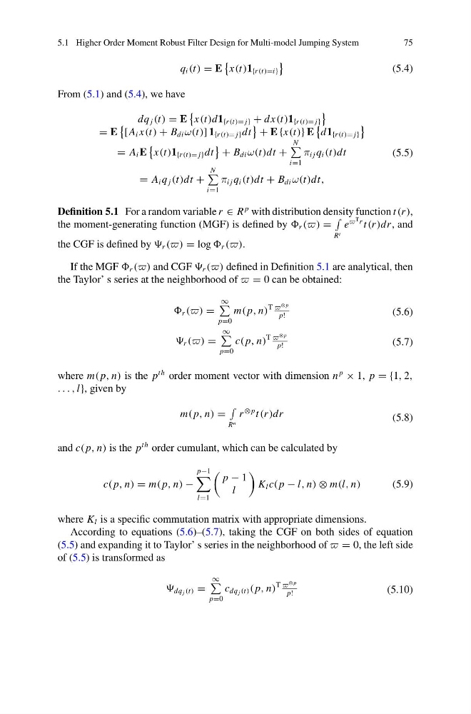
From (5.1) and (5.4), we have
dq j (t) = E
x(t)d1 {r (t)= j} + dx(t)1 {r (t)= j}
= E
[A i x(t) + B di ω(t)] 1 {r (t)= j} dt
+ E {x(t)} E
d1 {r (t)= j}
= A i E
x(t)1 {r (t)= j } dt
+ B di ω(t)dt +
N
i=1
π i j q i (t)dt
= A i q j (t)dt +
N
i=1
π i j q i (t)dt + B di ω(t)dt,
(5.5)
Definition 5.1 For a random variable r ∈ R
p with distribution density function t (r ),
the moment-generating function (MGF) is defined by r () =
R t
e
T r t (r )dr, and
the CGF is defined by r () = log r ().
If the MGF r () and CGF r () defined in Definition 5.1 are analytical, then
the Taylor’ s series at the neighborhood of = 0 can be obtained:
r () =
∞
p=0
m( p, n)
T
⊗ p
p!
(5.6)
r () =
∞
p=0
c( p, n)
T
⊗ p
p!
(5.7)
where m( p, n) is the p
th order moment vector with dimension n
p
× 1, p = {1, 2,
. . . , l}, given by
m( p, n) =
R n
r
⊗ p t (r )dr
(5.8)
and c( p, n) is the p
th order cumulant, which can be calculated by
c( p, n) = m( p, n) −
p−1
l=1
p − 1
l
K l c( p − l, n) ⊗ m(l, n)
(5.9)
where K l is a specific commutation matrix with appropriate dimensions.
According to equations (5.6)–(5.7), taking the CGF on both sides of equation
(5.5) and expanding it to Taylor’ s series in the neighborhood of = 0, the left side
of (5.5) is transformed as
dq j (t) =
∞
p=0
c dq j (t) ( p, n)
T
⊗ p
p!
(5.10)
75
q i (t) = E
x(t)1 {r (t)=i}
(5.4)
From (5.1) and (5.4), we have
dq j (t) = E
x(t)d1 {r (t)= j} + dx(t)1 {r (t)= j}
= E
[A i x(t) + B di ω(t)] 1 {r (t)= j} dt
+ E {x(t)} E
d1 {r (t)= j}
= A i E
x(t)1 {r (t)= j } dt
+ B di ω(t)dt +
N
i=1
π i j q i (t)dt
= A i q j (t)dt +
N
i=1
π i j q i (t)dt + B di ω(t)dt,
(5.5)
Definition 5.1 For a random variable r ∈ R
p with distribution density function t (r ),
the moment-generating function (MGF) is defined by r () =
R t
e
T r t (r )dr, and
the CGF is defined by r () = log r ().
If the MGF r () and CGF r () defined in Definition 5.1 are analytical, then
the Taylor’ s series at the neighborhood of = 0 can be obtained:
r () =
∞
p=0
m( p, n)
T
⊗ p
p!
(5.6)
r () =
∞
p=0
c( p, n)
T
⊗ p
p!
(5.7)
where m( p, n) is the p
th order moment vector with dimension n
p
× 1, p = {1, 2,
. . . , l}, given by
m( p, n) =
R n
r
⊗ p t (r )dr
(5.8)
and c( p, n) is the p
th order cumulant, which can be calculated by
c( p, n) = m( p, n) −
p−1
l=1
p − 1
l
K l c( p − l, n) ⊗ m(l, n)
(5.9)
where K l is a specific commutation matrix with appropriate dimensions.
According to equations (5.6)–(5.7), taking the CGF on both sides of equation
(5.5) and expanding it to Taylor’ s series in the neighborhood of = 0, the left side
of (5.5) is transformed as
dq j (t) =
∞
p=0
c dq j (t) ( p, n)
T
⊗ p
p!
(5.10)