

4.1 Robust Finite Frequency Filter Design for Multi-model Jumping System
53
dq j (t) = E
x(t)d1 {r (t)= j} + dx(t)1 {r (t)= j}
= E
[A i x(t) + B di ω(t)] 1 {r (t)= j } dt
+ E {x(t)} E
d1 {r (t)= j }
= A i E
x(t)1 {r (t)= j } dt
+ B di ω(t)dt +
N
i=1
π i j q i (t)dt
= A i q j (t)dt +
N
i=1
π i j q i (t)dt + B di ω(t)dt,
(4.4)
The above equation can be formed as
⎛
⎜
⎝
dq 1 (t)
. . .
dq N (t)
⎞
⎟
⎠ =
⎛
⎜
⎝
A 1 q 1 (t)
. . .
A N q N (t)
⎞
⎟
⎠ +
⎛
⎜
⎝
π 11 π 21 · · · π N 1
. . .
. . .
π 1N π 2N · · · π N N
⎞
⎟
⎠
⎛
⎜
⎝
q 1 (t)
. . .
q N (t)
⎞
⎟
⎠
+
⎛
⎜
⎝
B d1 ω(t)
. . .
B d N ω(t)
⎞
⎟
⎠
Define
q(t) =
q 1
T
(t) · · · q N
T
(t)
T ,
˜
y(t) =
y
T
(t) · · · y
T
(t)
T ,
˜
ω(t) =
ω
T
(t) · · · ω
T
(t)
T ,
˜
z(t) =
z
T
(t) · · · z
T
(t)
T .
Then, the multi-model jumping system defined in equation (4.1) can be transformed
to the following extended form:
⎧
⎨
⎩
˙
q(t) = Aq(t) + B d ˜
ω(t),
˜
y(t) = C 1 q(t) + D d ˜
ω(t),
˜
z(t) = C 2 q(t),
(4.5)
where A = diag{A 1 , A 2 , . . . , A N } +
T
⊗ I n ,
B d = diag{B d1 , B d2 , . . . , B d N },
C 1 = diag{C 11 , C 12 , . . . , C 1N },
C 2 = diag{C 21 , C 22 , . . . , C 2N },
D d = diag{D d1 , D d2 , . . . , D d N }.
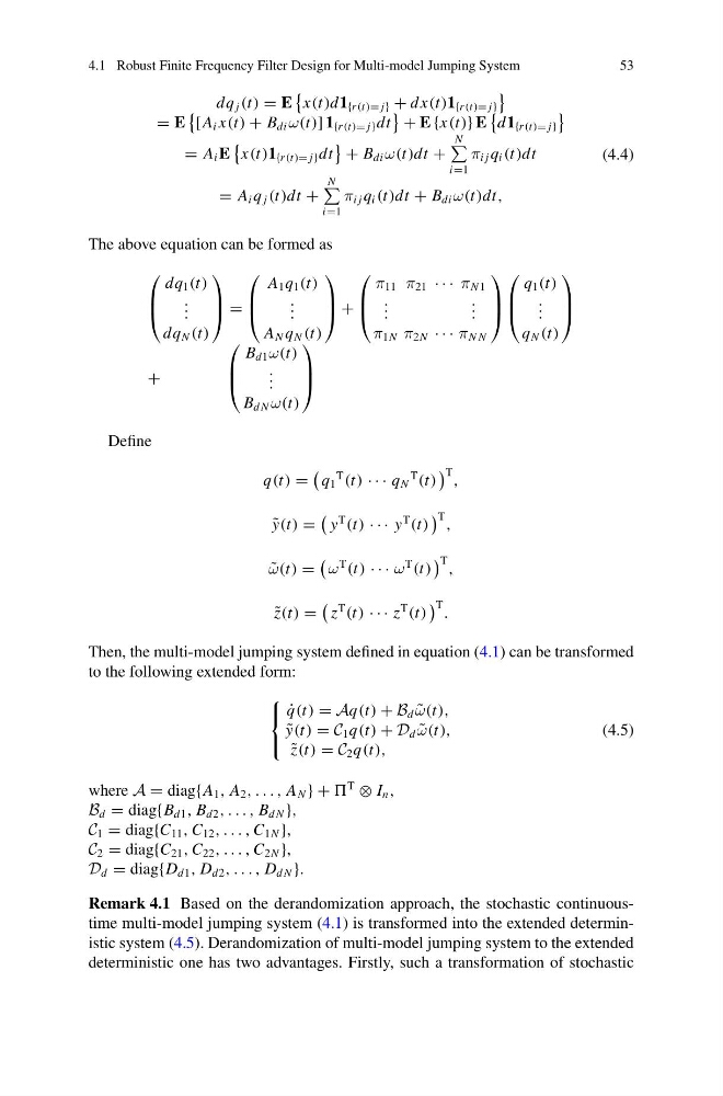
Remark 4.1 Based on the derandomization approach, the stochastic continuoustime multi-model jumping system (4.1) is transformed into the extended deterministic system (4.5). Derandomization of multi-model jumping system to the extended
deterministic one has two advantages. Firstly, such a transformation of stochastic
53
dq j (t) = E
x(t)d1 {r (t)= j} + dx(t)1 {r (t)= j}
= E
[A i x(t) + B di ω(t)] 1 {r (t)= j } dt
+ E {x(t)} E
d1 {r (t)= j }
= A i E
x(t)1 {r (t)= j } dt
+ B di ω(t)dt +
N
i=1
π i j q i (t)dt
= A i q j (t)dt +
N
i=1
π i j q i (t)dt + B di ω(t)dt,
(4.4)
The above equation can be formed as
⎛
⎜
⎝
dq 1 (t)
. . .
dq N (t)
⎞
⎟
⎠ =
⎛
⎜
⎝
A 1 q 1 (t)
. . .
A N q N (t)
⎞
⎟
⎠ +
⎛
⎜
⎝
π 11 π 21 · · · π N 1
. . .
. . .
π 1N π 2N · · · π N N
⎞
⎟
⎠
⎛
⎜
⎝
q 1 (t)
. . .
q N (t)
⎞
⎟
⎠
+
⎛
⎜
⎝
B d1 ω(t)
. . .
B d N ω(t)
⎞
⎟
⎠
Define
q(t) =
q 1
T
(t) · · · q N
T
(t)
T ,
˜
y(t) =
y
T
(t) · · · y
T
(t)
T ,
˜
ω(t) =
ω
T
(t) · · · ω
T
(t)
T ,
˜
z(t) =
z
T
(t) · · · z
T
(t)
T .
Then, the multi-model jumping system defined in equation (4.1) can be transformed
to the following extended form:
⎧
⎨
⎩
˙
q(t) = Aq(t) + B d ˜
ω(t),
˜
y(t) = C 1 q(t) + D d ˜
ω(t),
˜
z(t) = C 2 q(t),
(4.5)
where A = diag{A 1 , A 2 , . . . , A N } +
T
⊗ I n ,
B d = diag{B d1 , B d2 , . . . , B d N },
C 1 = diag{C 11 , C 12 , . . . , C 1N },
C 2 = diag{C 21 , C 22 , . . . , C 2N },
D d = diag{D d1 , D d2 , . . . , D d N }.
Remark 4.1 Based on the derandomization approach, the stochastic continuoustime multi-model jumping system (4.1) is transformed into the extended deterministic system (4.5). Derandomization of multi-model jumping system to the extended
deterministic one has two advantages. Firstly, such a transformation of stochastic