

3.1 Finite-Time Robust H ∞ Filtering for Multi-model Jumping System
37
i =
⎡
⎢
⎢
⎢
⎢
⎢
⎢
⎢
⎢
⎣
11i 12i 13i 0
15i
16i 17i
∗ 22i 23i 0
25i
26i 27i
∗
∗ 33i 0
0
0
0
∗
∗
∗ −Q
0
0
0
∗
∗
∗ ∗ −γ
2 e
−ηT I 0
0
∗
∗
∗ ∗
∗
−I 0
∗
∗
∗ ∗
∗
∗ −δ I
⎤
⎥
⎥
⎥
⎥
⎥
⎥
⎥
⎥
⎦
< 0
(3.33)
where
11i = 11i + δ i N
T
i N i ,
13i = 13i + δ i N
T
i N hi ,
17i = P i M i ,
27i = P i M i ,
33i = −Q + δ i N
T
hi N hi .
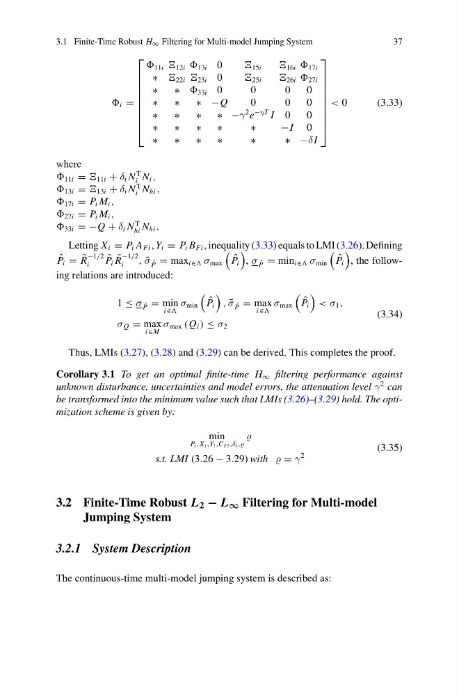
Letting X i = P i A Fi , Y i = P i B Fi , inequality (3.33) equals to LMI (3.26). Defining
ˆ
P i = ˜
R
−1/2
i
˜
P i ˜
R
−1/2
i
, ¯
σ ˆ
P = max i∈ σ max
ˆ
P i
, σ ˆ
P = min i∈ σ min
ˆ
P i
, the following relations are introduced:
1 ≤ σ ˆ
P = min
i∈
σ min
ˆ
P i
, ¯
σ ˆ
P = max
i∈
σ max
ˆ
P i
< σ 1 ,
σ Q = max
i∈M
σ max (Q i ) ≤ σ 2
(3.34)
Thus, LMIs (3.27), (3.28) and (3.29) can be derived. This completes the proof.
Corollary 3.1 To get an optimal finite-time H ∞ filtering performance against
unknown disturbance, uncertainties and model errors, the attenuation level γ
2 can
be transformed into the minimum value such that LMIs (3.26)–(3.29) hold. The optimization scheme is given by:
min
P i ,X i ,Y i ,C Fi ,δ i ,
s.t. LMI (3.26 − 3.29) with = γ
2
(3.35)
3.2 Finite-Time Robust L 2 − L ∞ Filtering for Multi-model
Jumping System
3.2.1 System Description
The continuous-time multi-model jumping system is described as:
37
i =
⎡
⎢
⎢
⎢
⎢
⎢
⎢
⎢
⎢
⎣
11i 12i 13i 0
15i
16i 17i
∗ 22i 23i 0
25i
26i 27i
∗
∗ 33i 0
0
0
0
∗
∗
∗ −Q
0
0
0
∗
∗
∗ ∗ −γ
2 e
−ηT I 0
0
∗
∗
∗ ∗
∗
−I 0
∗
∗
∗ ∗
∗
∗ −δ I
⎤
⎥
⎥
⎥
⎥
⎥
⎥
⎥
⎥
⎦
< 0
(3.33)
where
11i = 11i + δ i N
T
i N i ,
13i = 13i + δ i N
T
i N hi ,
17i = P i M i ,
27i = P i M i ,
33i = −Q + δ i N
T
hi N hi .
Letting X i = P i A Fi , Y i = P i B Fi , inequality (3.33) equals to LMI (3.26). Defining
ˆ
P i = ˜
R
−1/2
i
˜
P i ˜
R
−1/2
i
, ¯
σ ˆ
P = max i∈ σ max
ˆ
P i
, σ ˆ
P = min i∈ σ min
ˆ
P i
, the following relations are introduced:
1 ≤ σ ˆ
P = min
i∈
σ min
ˆ
P i
, ¯
σ ˆ
P = max
i∈
σ max
ˆ
P i
< σ 1 ,
σ Q = max
i∈M
σ max (Q i ) ≤ σ 2
(3.34)
Thus, LMIs (3.27), (3.28) and (3.29) can be derived. This completes the proof.
Corollary 3.1 To get an optimal finite-time H ∞ filtering performance against
unknown disturbance, uncertainties and model errors, the attenuation level γ
2 can
be transformed into the minimum value such that LMIs (3.26)–(3.29) hold. The optimization scheme is given by:
min
P i ,X i ,Y i ,C Fi ,δ i ,
s.t. LMI (3.26 − 3.29) with = γ
2
(3.35)
3.2 Finite-Time Robust L 2 − L ∞ Filtering for Multi-model
Jumping System
3.2.1 System Description
The continuous-time multi-model jumping system is described as: