

26
2 Robust Filtering for Multi-model Jumping System
Mode 1: A 1 =
−6 1.2
0.5 −7
, A h1 =
−5 0.2
0.3 −3.2
, B 1 =
0.3
0.2
, C 1 =
0.4 0.6
, C h1 =
0.3 0.4
, D 1 =
1
, L 1 =
0.3 0.1
, M 1 =
0.2
, N 1 =
0.3 0.1
.
Mode 2: A 2 =
−8.3 0.6
0.8 −6.7
, A h2 =
−8 0.3
0.5 −2
, B 2 =
0.5
0.3
, C 2 =
0.4 0.2
,
C h2 =
0.3 0.7
, D 2 =
2
, L 2 =
0.3 0.1
, M 2 =
0.4
, N 2 =
0.2 0.3
.
And the transition rate matrix is defined as:
=
−4 4
2 −2
.
By solving Theorem 2.1, we have ˜
γ min = 5.4281. Thus, the unbiased H ∞ filter
gain matrices are given by:
A F1 =
−8.8 −3
−2.3 −1.2
, A F2 =
−11.5 −1
−2.4 −8.3
, B F1 =
1.0791
−0.4473
,
B F2 =
0.8877
0.0492
, C F1 =
0.2523 0.0284
, C F2 =
0.1122 0.5561
, D F1 =
0.1194
, D F2 =
0.2196
.
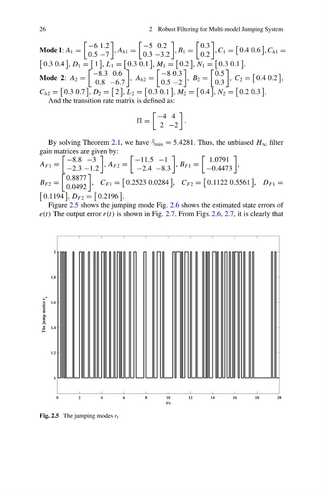
Figure 2.5 shows the jumping mode Fig. 2.6 shows the estimated state errors of
e(t) The output error r (t) is shown in Fig. 2.7. From Figs. 2.6, 2.7, it is clearly that
Fig. 2.5 The jumping modes r t
2 Robust Filtering for Multi-model Jumping System
Mode 1: A 1 =
−6 1.2
0.5 −7
, A h1 =
−5 0.2
0.3 −3.2
, B 1 =
0.3
0.2
, C 1 =
0.4 0.6
, C h1 =
0.3 0.4
, D 1 =
1
, L 1 =
0.3 0.1
, M 1 =
0.2
, N 1 =
0.3 0.1
.
Mode 2: A 2 =
−8.3 0.6
0.8 −6.7
, A h2 =
−8 0.3
0.5 −2
, B 2 =
0.5
0.3
, C 2 =
0.4 0.2
,
C h2 =
0.3 0.7
, D 2 =
2
, L 2 =
0.3 0.1
, M 2 =
0.4
, N 2 =
0.2 0.3
.
And the transition rate matrix is defined as:
=
−4 4
2 −2
.
By solving Theorem 2.1, we have ˜
γ min = 5.4281. Thus, the unbiased H ∞ filter
gain matrices are given by:
A F1 =
−8.8 −3
−2.3 −1.2
, A F2 =
−11.5 −1
−2.4 −8.3
, B F1 =
1.0791
−0.4473
,
B F2 =
0.8877
0.0492
, C F1 =
0.2523 0.0284
, C F2 =
0.1122 0.5561
, D F1 =
0.1194
, D F2 =
0.2196
.
Figure 2.5 shows the jumping mode Fig. 2.6 shows the estimated state errors of
e(t) The output error r (t) is shown in Fig. 2.7. From Figs. 2.6, 2.7, it is clearly that
Fig. 2.5 The jumping modes r t