

7.2 FDO Design for Fuzzy Multi-model Jumping System
129
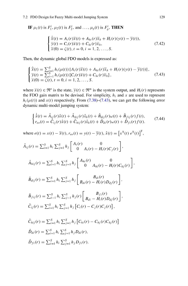
IF μ 1 (t) is F
i
1 , μ 2 (t) is F
i
2 , and . . . , μ g (t) is F
i
g , THEN
⎧
⎨
⎩
˙
x(t) = A i (r )x(t) + A hi (r )x h + H i (r )(y(t) − y(t)),
y(t) = C i (r )x(t) + C hi (r )x h ,
x(0) = ζ(t), t = 0, i = 1, 2, . . . , S.
(7.42)
Then, the dynamic global FDO models is expressed as:
⎧
⎨
⎩
˙
x(t) =
S
i=1 h i (μ(t)) [A i (r )x(t) + A hi (r )x h + H i (r )(y(t) − y(t))] ,
y(t) =
S
i=1 h i (μ(t)) [C i (r )x(t) + C hi (r )x h ] ,
x(0) = ζ(t), t = 0, i = 1, 2, . . . , S.
(7.43)
where x(t) ∈ R
n is the state, y(t) ∈ R
m is the system output, and H i (r ) represents
the FDO gain matrix to be devised. For simplicity, h i and x are used to represent
h i (μ(t)) and x(t) respectively. From (7.38)–(7.43), we can get the following error
dynamic multi-model jumping system:
˙ ˆ
x(t) = ˆ
A i j (r ) ˆ
x(t) + ˆ
A hi j (r ) ˆ
x h (t) + ˆ
B di j (r )ω(t) + ˆ
B f i j (r ) f (t),
r eo (t) = ˆ
C i j (r ) ˆ
x(t) + ˆ
C hi j (r ) ˆ
x h (t) + ˆ
D di (r )ω(t) + ˆ
D f i (r ) f (t).
(7.44)
where e(t) = x(t) − x(t), r eo (t) = y(t) − y(t), ˆ
x(t) =
x
T
(t) e
T
(t)
T ,
ˆ
A i j (r ) =
S
i=1 h i
S
j=1 h j
A i (r )
0
0 A i (r ) − H i (r )C j (r )
,
ˆ
A hi j (r ) =
S
i=1 h i
S
j=1 h j
A hi (r )
0
0 A hi (r ) − H i (r )C h j (r )
,
ˆ
B di j (r ) =
S
i=1 h i
S
j=1 h j
B di (r )
B di (r ) − H i (r )D d j (r )
,
ˆ
B f i j (r ) =
S
i=1 h i
S
j=1 h j (r )
B f i (r )
B di − H i (r )D d j (r )
,
ˆ
C i j (r ) =
S
i=1 h i
S
j=1 h j
C i (r ) − C j (r )C j (r )
,
ˆ
C hi j (r ) =
S
i=1 h i
S
j=1 h j
C hi (r ) − C h j (r )C h j (r )
ˆ
D di (r ) =
S
i=1 h i
S
j=1 h j D di (r ),
ˆ
D f i (r ) =
S
i=1 h i
S
j=1 h j D f i (r ).
129
IF μ 1 (t) is F
i
1 , μ 2 (t) is F
i
2 , and . . . , μ g (t) is F
i
g , THEN
⎧
⎨
⎩
˙
x(t) = A i (r )x(t) + A hi (r )x h + H i (r )(y(t) − y(t)),
y(t) = C i (r )x(t) + C hi (r )x h ,
x(0) = ζ(t), t = 0, i = 1, 2, . . . , S.
(7.42)
Then, the dynamic global FDO models is expressed as:
⎧
⎨
⎩
˙
x(t) =
S
i=1 h i (μ(t)) [A i (r )x(t) + A hi (r )x h + H i (r )(y(t) − y(t))] ,
y(t) =
S
i=1 h i (μ(t)) [C i (r )x(t) + C hi (r )x h ] ,
x(0) = ζ(t), t = 0, i = 1, 2, . . . , S.
(7.43)
where x(t) ∈ R
n is the state, y(t) ∈ R
m is the system output, and H i (r ) represents
the FDO gain matrix to be devised. For simplicity, h i and x are used to represent
h i (μ(t)) and x(t) respectively. From (7.38)–(7.43), we can get the following error
dynamic multi-model jumping system:
˙ ˆ
x(t) = ˆ
A i j (r ) ˆ
x(t) + ˆ
A hi j (r ) ˆ
x h (t) + ˆ
B di j (r )ω(t) + ˆ
B f i j (r ) f (t),
r eo (t) = ˆ
C i j (r ) ˆ
x(t) + ˆ
C hi j (r ) ˆ
x h (t) + ˆ
D di (r )ω(t) + ˆ
D f i (r ) f (t).
(7.44)
where e(t) = x(t) − x(t), r eo (t) = y(t) − y(t), ˆ
x(t) =
x
T
(t) e
T
(t)
T ,
ˆ
A i j (r ) =
S
i=1 h i
S
j=1 h j
A i (r )
0
0 A i (r ) − H i (r )C j (r )
,
ˆ
A hi j (r ) =
S
i=1 h i
S
j=1 h j
A hi (r )
0
0 A hi (r ) − H i (r )C h j (r )
,
ˆ
B di j (r ) =
S
i=1 h i
S
j=1 h j
B di (r )
B di (r ) − H i (r )D d j (r )
,
ˆ
B f i j (r ) =
S
i=1 h i
S
j=1 h j (r )
B f i (r )
B di − H i (r )D d j (r )
,
ˆ
C i j (r ) =
S
i=1 h i
S
j=1 h j
C i (r ) − C j (r )C j (r )
,
ˆ
C hi j (r ) =
S
i=1 h i
S
j=1 h j
C hi (r ) − C h j (r )C h j (r )
ˆ
D di (r ) =
S
i=1 h i
S
j=1 h j D di (r ),
ˆ
D f i (r ) =
S
i=1 h i
S
j=1 h j D f i (r ).