

66
4 Layout of a Single Floor
be the squared Euclidean distance between the centres of departments i and j . The
attractor component is the sum of the connectivities c ij multiplied by D ij :
ij
c ij D ij .
Possible choices for the repeller component are functions such as f (t) =
1
t or
f (t) = log(t) for which f (D ij ) → +∞ when D ij → 0.
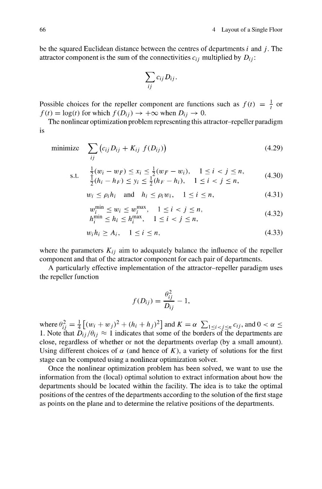
The nonlinear optimization problem representing this attractor–repeller paradigm
is
minimize
ij
c ij D ij + K ij f (D ij )
(4.29)
s.t.
1
2 (w i − w F ) ≤ x i ≤
1
2 (w F − w i ), 1 ≤ i < j ≤ n,
1
2 (h i − h F ) ≤ y i ≤
1
2 (h F − h i ), 1 ≤ i < j ≤ n,
(4.30)
w i ≤ ρ i h i and h i ≤ ρ i w i , 1 ≤ i ≤ n,
(4.31)
w min
i
≤ w i ≤ w
max
i
, 1 ≤ i < j ≤ n,
h min
i
≤ h i ≤ h max
i , 1 ≤ i < j ≤ n,
(4.32)
w i h i ≥ A i , 1 ≤ i ≤ n,
(4.33)
where the parameters K ij aim to adequately balance the influence of the repeller
component and that of the attractor component for each pair of departments.
A particularly effective implementation of the attractor–repeller paradigm uses
the repeller function
f (D ij ) =
θ 2
ij
D ij
− 1,
where θ 2
ij =
1
4
(w i + w j ) 2 + (h i + h j ) 2
and K = α
1≤i
close, regardless of whether or not the departments overlap (by a small amount).
Using different choices of α (and hence of K), a variety of solutions for the first
stage can be computed using a nonlinear optimization solver.
Once the nonlinear optimization problem has been solved, we want to use the
information from the (local) optimal solution to extract information about how the
departments should be located within the facility. The idea is to take the optimal
positions of the centres of the departments according to the solution of the first stage
as points on the plane and to determine the relative positions of the departments.
4 Layout of a Single Floor
be the squared Euclidean distance between the centres of departments i and j . The
attractor component is the sum of the connectivities c ij multiplied by D ij :
ij
c ij D ij .
Possible choices for the repeller component are functions such as f (t) =
1
t or
f (t) = log(t) for which f (D ij ) → +∞ when D ij → 0.
The nonlinear optimization problem representing this attractor–repeller paradigm
is
minimize
ij
c ij D ij + K ij f (D ij )
(4.29)
s.t.
1
2 (w i − w F ) ≤ x i ≤
1
2 (w F − w i ), 1 ≤ i < j ≤ n,
1
2 (h i − h F ) ≤ y i ≤
1
2 (h F − h i ), 1 ≤ i < j ≤ n,
(4.30)
w i ≤ ρ i h i and h i ≤ ρ i w i , 1 ≤ i ≤ n,
(4.31)
w min
i
≤ w i ≤ w
max
i
, 1 ≤ i < j ≤ n,
h min
i
≤ h i ≤ h max
i , 1 ≤ i < j ≤ n,
(4.32)
w i h i ≥ A i , 1 ≤ i ≤ n,
(4.33)
where the parameters K ij aim to adequately balance the influence of the repeller
component and that of the attractor component for each pair of departments.
A particularly effective implementation of the attractor–repeller paradigm uses
the repeller function
f (D ij ) =
θ 2
ij
D ij
− 1,
where θ 2
ij =
1
4
(w i + w j ) 2 + (h i + h j ) 2
and K = α
1≤i
close, regardless of whether or not the departments overlap (by a small amount).
Using different choices of α (and hence of K), a variety of solutions for the first
stage can be computed using a nonlinear optimization solver.
Once the nonlinear optimization problem has been solved, we want to use the
information from the (local) optimal solution to extract information about how the
departments should be located within the facility. The idea is to take the optimal
positions of the centres of the departments according to the solution of the first stage
as points on the plane and to determine the relative positions of the departments.