

2.7 Semidefinite Optimization Formulation
21
Without loss of generality, if we assume that i < j < k, then from (2.48) we have
α ki = 1 − α ik , α kj = 1 − α jk , and α ji = 1 − α ij . Substituting using these gives
α ij + α jk − α ik ≤ 1 and α ik − α jk − α ij ≤ 0, 1 ≤ i < j < k ≤ n.
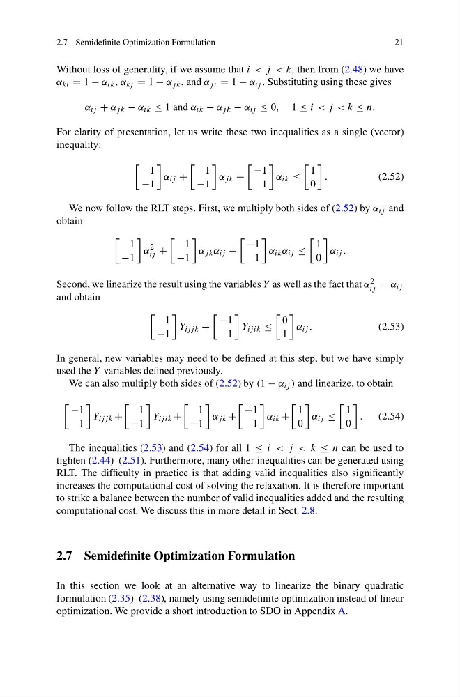
For clarity of presentation, let us write these two inequalities as a single (vector)
inequality:
1
−1
α ij +
1
−1
α jk +
−1
1
α ik ≤
1
0
.
(2.52)
We now follow the RLT steps. First, we multiply both sides of (2.52) by α ij and
obtain
1
−1
α
2
ij +
1
−1
α jk α ij +
−1
1
α ik α ij ≤
1
0
α ij .
Second, we linearize the result using the variables Y as well as the fact that α 2
ij = α ij
and obtain
1
−1
Y ijj k +
−1
1
Y ij ik ≤
0
1
α ij .
(2.53)
In general, new variables may need to be defined at this step, but we have simply
used the Y variables defined previously.
We can also multiply both sides of (2.52) by (1 − α ij ) and linearize, to obtain
−1
1
Y ijj k +
1
−1
Y ij ik +
1
−1
α jk +
−1
1
α ik +
1
0
α ij ≤
1
0
. (2.54)
The inequalities (2.53) and (2.54) for all 1 ≤ i < j < k ≤ n can be used to
tighten (2.44)–(2.51). Furthermore, many other inequalities can be generated using
RLT. The difficulty in practice is that adding valid inequalities also significantly
increases the computational cost of solving the relaxation. It is therefore important
to strike a balance between the number of valid inequalities added and the resulting
computational cost. We discuss this in more detail in Sect. 2.8.
2.7 Semidefinite Optimization Formulation
In this section we look at an alternative way to linearize the binary quadratic
formulation (2.35)–(2.38), namely using semidefinite optimization instead of linear
optimization. We provide a short introduction to SDO in Appendix A.
21
Without loss of generality, if we assume that i < j < k, then from (2.48) we have
α ki = 1 − α ik , α kj = 1 − α jk , and α ji = 1 − α ij . Substituting using these gives
α ij + α jk − α ik ≤ 1 and α ik − α jk − α ij ≤ 0, 1 ≤ i < j < k ≤ n.
For clarity of presentation, let us write these two inequalities as a single (vector)
inequality:
1
−1
α ij +
1
−1
α jk +
−1
1
α ik ≤
1
0
.
(2.52)
We now follow the RLT steps. First, we multiply both sides of (2.52) by α ij and
obtain
1
−1
α
2
ij +
1
−1
α jk α ij +
−1
1
α ik α ij ≤
1
0
α ij .
Second, we linearize the result using the variables Y as well as the fact that α 2
ij = α ij
and obtain
1
−1
Y ijj k +
−1
1
Y ij ik ≤
0
1
α ij .
(2.53)
In general, new variables may need to be defined at this step, but we have simply
used the Y variables defined previously.
We can also multiply both sides of (2.52) by (1 − α ij ) and linearize, to obtain
−1
1
Y ijj k +
1
−1
Y ij ik +
1
−1
α jk +
−1
1
α ik +
1
0
α ij ≤
1
0
. (2.54)
The inequalities (2.53) and (2.54) for all 1 ≤ i < j < k ≤ n can be used to
tighten (2.44)–(2.51). Furthermore, many other inequalities can be generated using
RLT. The difficulty in practice is that adding valid inequalities also significantly
increases the computational cost of solving the relaxation. It is therefore important
to strike a balance between the number of valid inequalities added and the resulting
computational cost. We discuss this in more detail in Sect. 2.8.
2.7 Semidefinite Optimization Formulation
In this section we look at an alternative way to linearize the binary quadratic
formulation (2.35)–(2.38), namely using semidefinite optimization instead of linear
optimization. We provide a short introduction to SDO in Appendix A.