18
2 Layout on a Single Row
Second, for any three distinct departments i, j, k, we enforce the transitivity
condition:
if i is to the left of j and j is to the left of k, then i is to the left of k.
In other words, if α ij = 1 and α jk = 1, then we must have α ik = 1 (or α ki = 0,
by 2.36). Equivalently, not all of α ij , α jk , and α ki may be equal to 1 simultaneously.
We express this using the constraints
α ij + α jk + α ki ≤ 2, 1 ≤ i = j = k ≤ n.
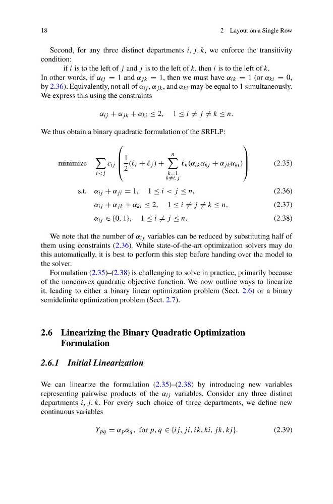
We thus obtain a binary quadratic formulation of the SRFLP:
minimize
i c ij
⎛
⎜
⎜
⎝
1
2
(( i + j ) +
n
k=1
k =i,j
k (α ik α kj + α jk α ki )
⎞
⎟
⎟
⎠
(2.35)
s.t. α ij + α ji = 1, 1 ≤ i < j ≤ n,
(2.36)
α ij + α jk + α ki ≤ 2, 1 ≤ i = j = k ≤ n,
(2.37)
α ij ∈ {0, 1}, 1 ≤ i = j ≤ n.
(2.38)
We note that the number of α ij variables can be reduced by substituting half of
them using constraints (2.36). While state-of-the-art optimization solvers may do
this automatically, it is best to perform this step before handing over the model to
the solver.
Formulation (2.35)–(2.38) is challenging to solve in practice, primarily because
of the nonconvex quadratic objective function. We now outline ways to linearize
it, leading to either a binary linear optimization problem (Sect. 2.6) or a binary
semidefinite optimization problem (Sect. 2.7).
2.6 Linearizing the Binary Quadratic Optimization
Formulation
2.6.1 Initial Linearization
We can linearize the formulation (2.35)–(2.38) by introducing new variables
representing pairwise products of the α ij variables. Consider any three distinct
departments i, j, k. For every such choice of three departments, we define new
continuous variables
Y pq = α p α q , for p, q ∈ {ij, j i, ik, ki, j k, kj }.
(2.39)