

2.1 Introductory Example
5
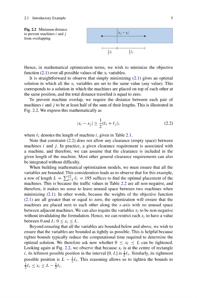
Fig. 2.2 Minimum distance
to prevent machines i and j
from overlapping
1
2 l i
1
2 l j
|x j x i |
Hence, in mathematical optimization terms, we wish to minimize the objective
function (2.1) over all possible values of the x i variables.
It is straightforward to observe that simply minimizing (2.1) gives an optimal
solution in which all the x i variables are set to the same value (any value). This
corresponds to a solution in which the machines are placed on top of each other at
the same position, and the total distance travelled is equal to zero.
To prevent machine overlap, we require the distance between each pair of
machines i and j to be at least half of the sum of their lengths. This is illustrated in
Fig. 2.2. We express this mathematically as
|x i − x j | ≥
1
2
(( i + j ),
(2.2)
where i denotes the length of machine i, given in Table 2.1.
Note that constraint (2.2) does not allow any clearance (empty space) between
machines i and j . In practice, a given clearance requirement is associated with
a machine, and therefore, we can assume that the clearance is included in the
given length of the machine. Most other general clearance requirements can also
be integrated without difficulty.
When building mathematical optimization models, we must ensure that all the
variables are bounded. This consideration leads us to observe that for this example,
a row of length L =
12
i=1 i = 195 suffices to find the optimal placement of the
machines. This is because the traffic values in Table 2.2 are all non-negative, and
therefore, it makes no sense to leave unused space between two machines when
minimizing (2.1). In other words, because the weights of the objective function
(2.1) are all greater than or equal to zero, the optimization will ensure that the
machines are placed next to each other along the x-axis with no unused space
between adjacent machines. We can also require the variables x i to be non-negative
without invalidating the formulation. Hence, we can restrict each x i to have a value
between 0 and L: 0 ≤ x i ≤ L.
Beyond ensuring that all the variables are bounded below and above, we wish to
ensure that the variables are bounded as tightly as possible. This is helpful because
tighter bounds typically reduce the computational time required to determine the
optimal solution. We therefore ask now whether 0 ≤ x i ≤ L can be tightened.
Looking again at Fig. 2.2, we observe that because x i is at the centre of rectangle
i, its leftmost possible position in the interval [0, L] is
1
2 i . Similarly, its rightmost
possible position is L −
1
2 i . This reasoning allows us to tighten the bounds to
1
2 i ≤ x i ≤ L −
1
2 i .
5
Fig. 2.2 Minimum distance
to prevent machines i and j
from overlapping
1
2 l i
1
2 l j
|x j x i |
Hence, in mathematical optimization terms, we wish to minimize the objective
function (2.1) over all possible values of the x i variables.
It is straightforward to observe that simply minimizing (2.1) gives an optimal
solution in which all the x i variables are set to the same value (any value). This
corresponds to a solution in which the machines are placed on top of each other at
the same position, and the total distance travelled is equal to zero.
To prevent machine overlap, we require the distance between each pair of
machines i and j to be at least half of the sum of their lengths. This is illustrated in
Fig. 2.2. We express this mathematically as
|x i − x j | ≥
1
2
(( i + j ),
(2.2)
where i denotes the length of machine i, given in Table 2.1.
Note that constraint (2.2) does not allow any clearance (empty space) between
machines i and j . In practice, a given clearance requirement is associated with
a machine, and therefore, we can assume that the clearance is included in the
given length of the machine. Most other general clearance requirements can also
be integrated without difficulty.
When building mathematical optimization models, we must ensure that all the
variables are bounded. This consideration leads us to observe that for this example,
a row of length L =
12
i=1 i = 195 suffices to find the optimal placement of the
machines. This is because the traffic values in Table 2.2 are all non-negative, and
therefore, it makes no sense to leave unused space between two machines when
minimizing (2.1). In other words, because the weights of the objective function
(2.1) are all greater than or equal to zero, the optimization will ensure that the
machines are placed next to each other along the x-axis with no unused space
between adjacent machines. We can also require the variables x i to be non-negative
without invalidating the formulation. Hence, we can restrict each x i to have a value
between 0 and L: 0 ≤ x i ≤ L.
Beyond ensuring that all the variables are bounded below and above, we wish to
ensure that the variables are bounded as tightly as possible. This is helpful because
tighter bounds typically reduce the computational time required to determine the
optimal solution. We therefore ask now whether 0 ≤ x i ≤ L can be tightened.
Looking again at Fig. 2.2, we observe that because x i is at the centre of rectangle
i, its leftmost possible position in the interval [0, L] is
1
2 i . Similarly, its rightmost
possible position is L −
1
2 i . This reasoning allows us to tighten the bounds to
1
2 i ≤ x i ≤ L −
1
2 i .