

6.7 Colligative Properties
293
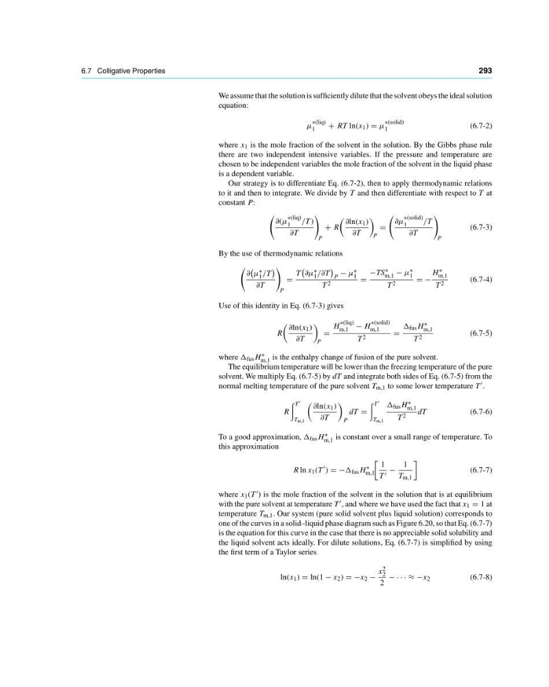
We assume that the solution is sufficiently dilute that the solvent obeys the ideal solution
equation:
µ
∗(liq)
1
+ RT ln(x 1 ) µ
∗(solid)
1
(6.7-2)
where x 1 is the mole fraction of the solvent in the solution. By the Gibbs phase rule
there are two independent intensive variables. If the pressure and temperature are
chosen to be independent variables the mole fraction of the solvent in the liquid phase
is a dependent variable.
Our strategy is to differentiate Eq. (6.7-2), then to apply thermodynamic relations
to it and then to integrate. We divide by T and then differentiate with respect to T at
constant P:
∂(µ
∗(liq)
1
/T )
∂T
P
+ R
∂ln(x 1 )
∂T
P
∂µ
∗(solid)
1
/T
∂T
P
(6.7-3)
By the use of thermodynamic relations
∂
µ ∗
1 /T
∂T
P
T
∂µ ∗
1 /∂T
P
− µ ∗
1
T 2
−TS ∗
m,1 − µ ∗
1
T 2
−
H ∗
m,1
T 2
(6.7-4)
Use of this identity in Eq. (6.7-3) gives
R
∂ln(x 1 )
∂T
P
H
∗(liq)
m,1 − H
∗(solid)
m,1
T 2
∆ fus H ∗
m,1
T 2
(6.7-5)
where ∆ fus H ∗
m,1 is the enthalpy change of fusion of the pure solvent.
The equilibrium temperature will be lower than the freezing temperature of the pure
solvent. We multiply Eq. (6.7-5) by dT and integrate both sides of Eq. (6.7-5) from the
normal melting temperature of the pure solvent T m,1 to some lower temperature T .
R
T
T m,1
∂ln(x 1 )
∂T
P
dT
T
T m,1
∆ fus H ∗
m,1
T 2 dT
(6.7-6)
To a good approximation, ∆ fus H ∗
m,1 is constant over a small range of temperature. To
this approximation
R ln x 1 (T
) −∆ fus H
∗
m,1
1
T −
1
T m,1
(6.7-7)
where x 1 (T ) is the mole fraction of the solvent in the solution that is at equilibrium
with the pure solvent at temperature T , and where we have used the fact that x 1 1 at
temperature T m,1 . Our system (pure solid solvent plus liquid solution) corresponds to
one of the curves in a solid–liquid phase diagram such as Figure 6.20, so that Eq. (6.7-7)
is the equation for this curve in the case that there is no appreciable solid solubility and
the liquid solvent acts ideally. For dilute solutions, Eq. (6.7-7) is simplified by using
the first term of a Taylor series
ln(x 1 ) ln(1 − x 2 ) −x 2 −
x 2
2
2
− · · · ≈ −x 2
(6.7-8)
293
We assume that the solution is sufficiently dilute that the solvent obeys the ideal solution
equation:
µ
∗(liq)
1
+ RT ln(x 1 ) µ
∗(solid)
1
(6.7-2)
where x 1 is the mole fraction of the solvent in the solution. By the Gibbs phase rule
there are two independent intensive variables. If the pressure and temperature are
chosen to be independent variables the mole fraction of the solvent in the liquid phase
is a dependent variable.
Our strategy is to differentiate Eq. (6.7-2), then to apply thermodynamic relations
to it and then to integrate. We divide by T and then differentiate with respect to T at
constant P:
∂(µ
∗(liq)
1
/T )
∂T
P
+ R
∂ln(x 1 )
∂T
P
∂µ
∗(solid)
1
/T
∂T
P
(6.7-3)
By the use of thermodynamic relations
∂
µ ∗
1 /T
∂T
P
T
∂µ ∗
1 /∂T
P
− µ ∗
1
T 2
−TS ∗
m,1 − µ ∗
1
T 2
−
H ∗
m,1
T 2
(6.7-4)
Use of this identity in Eq. (6.7-3) gives
R
∂ln(x 1 )
∂T
P
H
∗(liq)
m,1 − H
∗(solid)
m,1
T 2
∆ fus H ∗
m,1
T 2
(6.7-5)
where ∆ fus H ∗
m,1 is the enthalpy change of fusion of the pure solvent.
The equilibrium temperature will be lower than the freezing temperature of the pure
solvent. We multiply Eq. (6.7-5) by dT and integrate both sides of Eq. (6.7-5) from the
normal melting temperature of the pure solvent T m,1 to some lower temperature T .
R
T
T m,1
∂ln(x 1 )
∂T
P
dT
T
T m,1
∆ fus H ∗
m,1
T 2 dT
(6.7-6)
To a good approximation, ∆ fus H ∗
m,1 is constant over a small range of temperature. To
this approximation
R ln x 1 (T
) −∆ fus H
∗
m,1
1
T −
1
T m,1
(6.7-7)
where x 1 (T ) is the mole fraction of the solvent in the solution that is at equilibrium
with the pure solvent at temperature T , and where we have used the fact that x 1 1 at
temperature T m,1 . Our system (pure solid solvent plus liquid solution) corresponds to
one of the curves in a solid–liquid phase diagram such as Figure 6.20, so that Eq. (6.7-7)
is the equation for this curve in the case that there is no appreciable solid solubility and
the liquid solvent acts ideally. For dilute solutions, Eq. (6.7-7) is simplified by using
the first term of a Taylor series
ln(x 1 ) ln(1 − x 2 ) −x 2 −
x 2
2
2
− · · · ≈ −x 2
(6.7-8)