

6.1 Ideal Solutions
245
If the pressure is taken as an independent variable, the mole fractions in the two phases,
represented by the ends of the tie line, are dependent variables.
Temperature–Composition Phase Diagrams
In this type of phase diagram the pressure is held fixed. For two components the mole
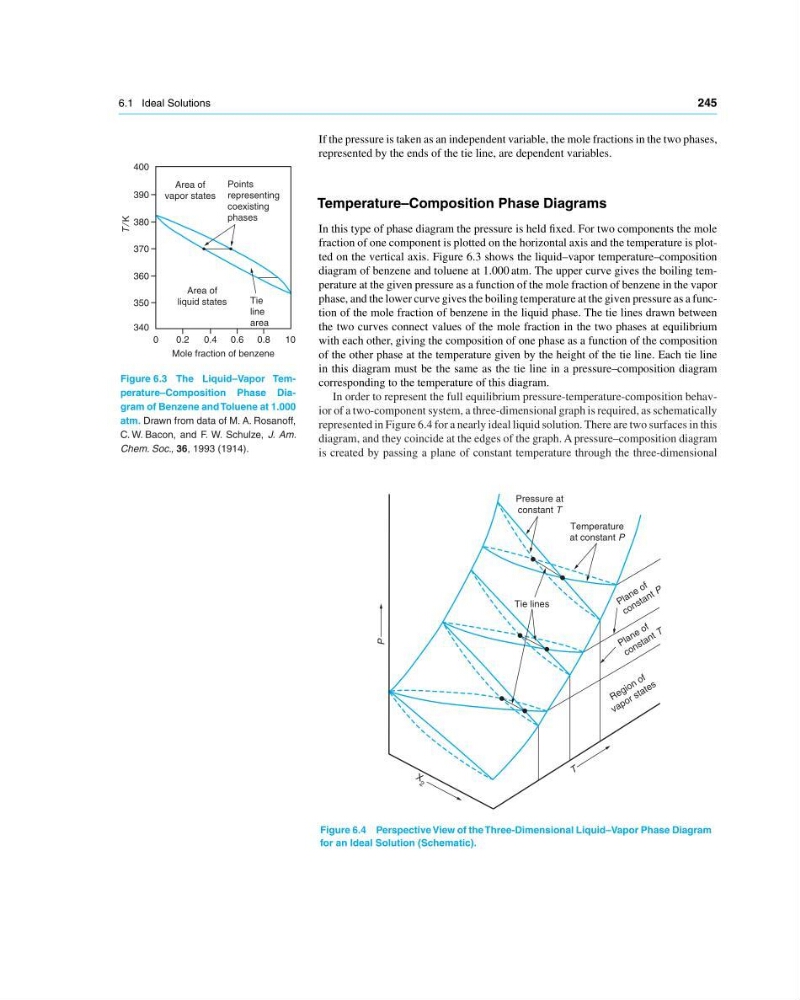
fraction of one component is plotted on the horizontal axis and the temperature is plotted on the vertical axis. Figure 6.3 shows the liquid–vapor temperature–composition
diagram of benzene and toluene at 1.000 atm. The upper curve gives the boiling temperature at the given pressure as a function of the mole fraction of benzene in the vapor
phase, and the lower curve gives the boiling temperature at the given pressure as a function of the mole fraction of benzene in the liquid phase. The tie lines drawn between
the two curves connect values of the mole fraction in the two phases at equilibrium
with each other, giving the composition of one phase as a function of the composition
of the other phase at the temperature given by the height of the tie line. Each tie line
in this diagram must be the same as the tie line in a pressure–composition diagram
corresponding to the temperature of this diagram.
Area of
vapor states
400
390
380
370
360
350
340
0
0.2
0.4 0.6 0.8
10
Mole fraction of benzene
T/ K
Area of
liquid states
Tie
line
area
Points
representing
coexisting
phases
Figure 6.3 The Liquid–Vapor Temperature–Composition Phase Diagram of Benzene and Toluene at 1.000
atm. Drawn from data of M. A. Rosanoff,
C. W. Bacon, and F. W. Schulze, J. Am.
Chem. Soc., 36, 1993 (1914).
In order to represent the full equilibrium pressure-temperature-composition behavior of a two-component system, a three-dimensional graph is required, as schematically
represented in Figure 6.4 for a nearly ideal liquid solution. There are two surfaces in this
diagram, and they coincide at the edges of the graph. A pressure–composition diagram
is created by passing a plane of constant temperature through the three-dimensional
Pressure at
constant T
Temperature
at constant P
Tie lines
P la n e o f
c o n s t a n t P
P la n e o f
c o n s t a n t T
R e g io n o f
v a p o r s t a t e s
T
X
2
P
Figure 6.4 Perspective View of the Three-Dimensional Liquid–Vapor Phase Diagram
for an Ideal Solution (Schematic).
245
If the pressure is taken as an independent variable, the mole fractions in the two phases,
represented by the ends of the tie line, are dependent variables.
Temperature–Composition Phase Diagrams
In this type of phase diagram the pressure is held fixed. For two components the mole
fraction of one component is plotted on the horizontal axis and the temperature is plotted on the vertical axis. Figure 6.3 shows the liquid–vapor temperature–composition
diagram of benzene and toluene at 1.000 atm. The upper curve gives the boiling temperature at the given pressure as a function of the mole fraction of benzene in the vapor
phase, and the lower curve gives the boiling temperature at the given pressure as a function of the mole fraction of benzene in the liquid phase. The tie lines drawn between
the two curves connect values of the mole fraction in the two phases at equilibrium
with each other, giving the composition of one phase as a function of the composition
of the other phase at the temperature given by the height of the tie line. Each tie line
in this diagram must be the same as the tie line in a pressure–composition diagram
corresponding to the temperature of this diagram.
Area of
vapor states
400
390
380
370
360
350
340
0
0.2
0.4 0.6 0.8
10
Mole fraction of benzene
T/ K
Area of
liquid states
Tie
line
area
Points
representing
coexisting
phases
Figure 6.3 The Liquid–Vapor Temperature–Composition Phase Diagram of Benzene and Toluene at 1.000
atm. Drawn from data of M. A. Rosanoff,
C. W. Bacon, and F. W. Schulze, J. Am.
Chem. Soc., 36, 1993 (1914).
In order to represent the full equilibrium pressure-temperature-composition behavior of a two-component system, a three-dimensional graph is required, as schematically
represented in Figure 6.4 for a nearly ideal liquid solution. There are two surfaces in this
diagram, and they coincide at the edges of the graph. A pressure–composition diagram
is created by passing a plane of constant temperature through the three-dimensional
Pressure at
constant T
Temperature
at constant P
Tie lines
P la n e o f
c o n s t a n t P
P la n e o f
c o n s t a n t T
R e g io n o f
v a p o r s t a t e s
T
X
2
P
Figure 6.4 Perspective View of the Three-Dimensional Liquid–Vapor Phase Diagram
for an Ideal Solution (Schematic).