

270
D. Escudero
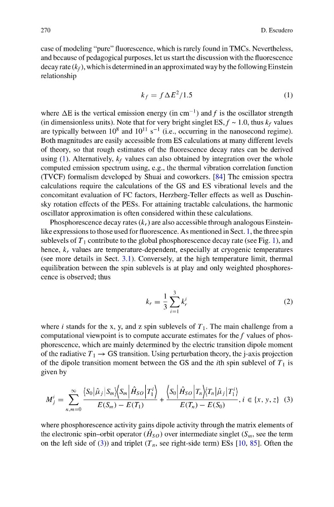
case of modeling “pure” fluorescence, which is rarely found in TMCs. Nevertheless,
and because of pedagogical purposes, let us start the discussion with the fluorescence
decay rate (k f ), which is determined in an approximated way by the following Einstein
relationship
k f f E
2
/1.5
( 1 )
where E is the vertical emission energy (in cm
−1 ) and f is the oscillator strength
(in dimensionless units). Note that for very bright singlet ES, f ~ 1.0, thus k f values
are typically between 10
8 and 10
11 s
−1 (i.e., occurring in the nanosecond regime).
Both magnitudes are easily accessible from ES calculations at many different levels
of theory, so that rough estimates of the fluorescence decay rates can be derived
using (1). Alternatively, k f values can also obtained by integration over the whole
computed emission spectrum using, e.g., the thermal vibration correlation function
(TVCF) formalism developed by Shuai and coworkers. [84] The emission spectra
calculations require the calculations of the GS and ES vibrational levels and the
concomitant evaluation of FC factors, Herzberg-Teller effects as well as Duschinsky rotation effects of the PESs. For attaining tractable calculations, the harmonic
oscillator approximation is often considered within these calculations.
Phosphorescence decay rates (k r ) are also accessible through analogous Einsteinlike expressions to those used for fluorescence. As mentioned in Sect. 1, the three spin
sublevels of T 1 contribute to the global phosphorescence decay rate (see Fig. 1), and
hence, k r values are temperature-dependent, especially at cryogenic temperatures
(see more details in Sect. 3.1). Conversely, at the high temperature limit, thermal
equilibration between the spin sublevels is at play and only weighted phosphorescence is observed; thus
k r
1
3
3
i1
k
i
r
(2)
where i stands for the x, y, and z spin sublevels of T 1 . The main challenge from a
computational viewpoint is to compute accurate estimates for the f values of phosphorescence, which are mainly determined by the electric transition dipole moment
of the radiative T 1 → GS transition. Using perturbation theory, the j-axis projection
of the dipole transition moment between the GS and the ith spin sublevel of T 1 is
given by
M
i
j
∞
n,m0
S 0
ˆ
μ j
S m
S m
ˆ
H SO
T
i
1
E(S m ) − E(T 1 )
+
S 0
ˆ
H SO
Tn
T n
ˆ
μ j
T
i
1
E(T n ) − E(S 0 )
, i ∈ {x, y, z} (3)
where phosphorescence activity gains dipole activity through the matrix elements of
the electronic spin–orbit operator ( ˆ
H SO ) over intermediate singlet (S m , see the term
on the left side of (3)) and triplet (T n , see right-side term) ESs [10, 85]. Often the
D. Escudero
case of modeling “pure” fluorescence, which is rarely found in TMCs. Nevertheless,
and because of pedagogical purposes, let us start the discussion with the fluorescence
decay rate (k f ), which is determined in an approximated way by the following Einstein
relationship
k f f E
2
/1.5
( 1 )
where E is the vertical emission energy (in cm
−1 ) and f is the oscillator strength
(in dimensionless units). Note that for very bright singlet ES, f ~ 1.0, thus k f values
are typically between 10
8 and 10
11 s
−1 (i.e., occurring in the nanosecond regime).
Both magnitudes are easily accessible from ES calculations at many different levels
of theory, so that rough estimates of the fluorescence decay rates can be derived
using (1). Alternatively, k f values can also obtained by integration over the whole
computed emission spectrum using, e.g., the thermal vibration correlation function
(TVCF) formalism developed by Shuai and coworkers. [84] The emission spectra
calculations require the calculations of the GS and ES vibrational levels and the
concomitant evaluation of FC factors, Herzberg-Teller effects as well as Duschinsky rotation effects of the PESs. For attaining tractable calculations, the harmonic
oscillator approximation is often considered within these calculations.
Phosphorescence decay rates (k r ) are also accessible through analogous Einsteinlike expressions to those used for fluorescence. As mentioned in Sect. 1, the three spin
sublevels of T 1 contribute to the global phosphorescence decay rate (see Fig. 1), and
hence, k r values are temperature-dependent, especially at cryogenic temperatures
(see more details in Sect. 3.1). Conversely, at the high temperature limit, thermal
equilibration between the spin sublevels is at play and only weighted phosphorescence is observed; thus
k r
1
3
3
i1
k
i
r
(2)
where i stands for the x, y, and z spin sublevels of T 1 . The main challenge from a
computational viewpoint is to compute accurate estimates for the f values of phosphorescence, which are mainly determined by the electric transition dipole moment
of the radiative T 1 → GS transition. Using perturbation theory, the j-axis projection
of the dipole transition moment between the GS and the ith spin sublevel of T 1 is
given by
M
i
j
∞
n,m0
S 0
ˆ
μ j
S m
S m
ˆ
H SO
T
i
1
E(S m ) − E(T 1 )
+
S 0
ˆ
H SO
Tn
T n
ˆ
μ j
T
i
1
E(T n ) − E(S 0 )
, i ∈ {x, y, z} (3)
where phosphorescence activity gains dipole activity through the matrix elements of
the electronic spin–orbit operator ( ˆ
H SO ) over intermediate singlet (S m , see the term
on the left side of (3)) and triplet (T n , see right-side term) ESs [10, 85]. Often the