

Multiconfigurational Approach to X-ray Spectroscopy …
191
3.2 Active-Space Selection
The second step in the design of the calculation is the choice of the active space, the
trademark of multiconfigurational methods. The general rules for any application
are to include in the active space any orbital participating in strong correlation. For
electronic excitations, any orbital whose occupation is expected to change significantly should also be included. In practice, this selection requires both expertise and
experience. Aiming at making multiconfigurational calculations more black box,
there have been developments toward automated active-space selection where the
selection criteria are meant to optimize the description of strong correlation [83].
However, such criteria cannot be directly applied to spectrum calculations as the
orbitals important to describe the photoexcitation process are not necessarily the
same that contribute most to correlation. In practice, the final choice of active space
is still driven by chemical intuition and experience.
For transition metals, there is a wealth of experience on the choice of active
space to describe strong correlation and intuitive rules have been compiled [69]. For
X-ray spectroscopy, where the range of final states span over several eV, the target
accuracy is typically lower than most other applications and the active space can be
reduced somewhat. One can often satisfactorily restrict the selection to the metal
3d orbitals and any ligand orbitals forming strong covalent bonds with the metal.
Local symmetry, either strict or approximate, can significantly help reducing the
number of ligand orbitals included. To this space, one should add orbitals that are
excited to or from in the X-ray process, which typically are virtual orbitals with
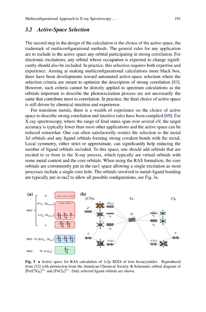
some metal content and the core orbitals. When using the RAS formalism, the core
orbitals are conveniently put in the ras1 space allowing a single excitation as most
processes include a single core hole. The orbitals involved in metal–ligand bonding
are typically put in ras2 to allow all possible configurations, see Fig. 3a.
Fig. 3 a Active space for RAS calculation of 1s2p RIXS of iron hexacyanides. Reproduced
from [32] with permission from the American Chemical Society. b Schematic orbital diagram of
[Fe(CN) 6 ] 3− and [FeCl 6 ] 3− . Only selected ligand orbitals are shown
191
3.2 Active-Space Selection
The second step in the design of the calculation is the choice of the active space, the
trademark of multiconfigurational methods. The general rules for any application
are to include in the active space any orbital participating in strong correlation. For
electronic excitations, any orbital whose occupation is expected to change significantly should also be included. In practice, this selection requires both expertise and
experience. Aiming at making multiconfigurational calculations more black box,
there have been developments toward automated active-space selection where the
selection criteria are meant to optimize the description of strong correlation [83].
However, such criteria cannot be directly applied to spectrum calculations as the
orbitals important to describe the photoexcitation process are not necessarily the
same that contribute most to correlation. In practice, the final choice of active space
is still driven by chemical intuition and experience.
For transition metals, there is a wealth of experience on the choice of active
space to describe strong correlation and intuitive rules have been compiled [69]. For
X-ray spectroscopy, where the range of final states span over several eV, the target
accuracy is typically lower than most other applications and the active space can be
reduced somewhat. One can often satisfactorily restrict the selection to the metal
3d orbitals and any ligand orbitals forming strong covalent bonds with the metal.
Local symmetry, either strict or approximate, can significantly help reducing the
number of ligand orbitals included. To this space, one should add orbitals that are
excited to or from in the X-ray process, which typically are virtual orbitals with
some metal content and the core orbitals. When using the RAS formalism, the core
orbitals are conveniently put in the ras1 space allowing a single excitation as most
processes include a single core hole. The orbitals involved in metal–ligand bonding
are typically put in ras2 to allow all possible configurations, see Fig. 3a.
Fig. 3 a Active space for RAS calculation of 1s2p RIXS of iron hexacyanides. Reproduced
from [32] with permission from the American Chemical Society. b Schematic orbital diagram of
[Fe(CN) 6 ] 3− and [FeCl 6 ] 3− . Only selected ligand orbitals are shown