

256
17 Coupled-Cluster Methods for Generalized Excitations
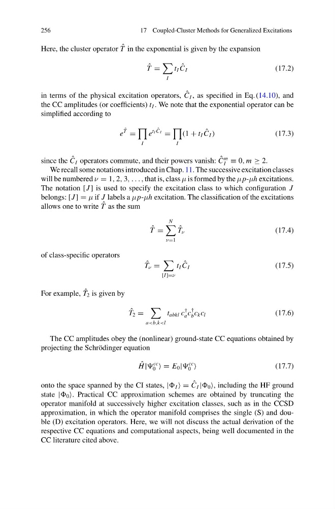
Here, the cluster operator ˆ
T in the exponential is given by the expansion
ˆ
T =
I
t I ˆ
C I
(17.2)
in terms of the physical excitation operators, ˆ
C I , as specified in Eq. (14.10), and
the CC amplitudes (or coefficients) t I . We note that the exponential operator can be
simplified according to
e
ˆ
T
=
I
e
t I ˆ
C I =
I
(1 + t I ˆ
C I )
(17.3)
since the ˆ
C I operators commute, and their powers vanish: ˆ
C
m
I ≡ 0, m ≥ 2.
We recall some notations introduced in Chap. 11. The successive excitation classes
will be numbered ν = 1, 2, 3, . . . , that is, class μ is formed by the μ p-μh excitations.
The notation [J ] is used to specify the excitation class to which configuration J
belongs: [J ] = μ if J labels a μ p-μh excitation. The classification of the excitations
allows one to write ˆ
T as the sum
ˆ
T =
N
ν=1
ˆ
T ν
(17.4)
of class-specific operators
ˆ
T ν =
[I ]=ν
t I ˆ
C I
(17.5)
For example, ˆ
T 2 is given by
ˆ
T 2 =
a
†
a c
†
b c k c l
(17.6)
The CC amplitudes obey the (nonlinear) ground-state CC equations obtained by
projecting the Schrödinger equation
ˆ
H |
cc
0 = E 0 |
cc
0
(17.7)
onto the space spanned by the CI states, | I = ˆ
C I | 0 , including the HF ground
state | 0 . Practical CC approximation schemes are obtained by truncating the
operator manifold at successively higher excitation classes, such as in the CCSD
approximation, in which the operator manifold comprises the single (S) and double (D) excitation operators. Here, we will not discuss the actual derivation of the
respective CC equations and computational aspects, being well documented in the
CC literature cited above.
17 Coupled-Cluster Methods for Generalized Excitations
Here, the cluster operator ˆ
T in the exponential is given by the expansion
ˆ
T =
I
t I ˆ
C I
(17.2)
in terms of the physical excitation operators, ˆ
C I , as specified in Eq. (14.10), and
the CC amplitudes (or coefficients) t I . We note that the exponential operator can be
simplified according to
e
ˆ
T
=
I
e
t I ˆ
C I =
I
(1 + t I ˆ
C I )
(17.3)
since the ˆ
C I operators commute, and their powers vanish: ˆ
C
m
I ≡ 0, m ≥ 2.
We recall some notations introduced in Chap. 11. The successive excitation classes
will be numbered ν = 1, 2, 3, . . . , that is, class μ is formed by the μ p-μh excitations.
The notation [J ] is used to specify the excitation class to which configuration J
belongs: [J ] = μ if J labels a μ p-μh excitation. The classification of the excitations
allows one to write ˆ
T as the sum
ˆ
T =
N
ν=1
ˆ
T ν
(17.4)
of class-specific operators
ˆ
T ν =
[I ]=ν
t I ˆ
C I
(17.5)
For example, ˆ
T 2 is given by
ˆ
T 2 =
a
†
a c
†
b c k c l
(17.6)
The CC amplitudes obey the (nonlinear) ground-state CC equations obtained by
projecting the Schrödinger equation
ˆ
H |
cc
0 = E 0 |
cc
0
(17.7)
onto the space spanned by the CI states, | I = ˆ
C I | 0 , including the HF ground
state | 0 . Practical CC approximation schemes are obtained by truncating the
operator manifold at successively higher excitation classes, such as in the CCSD
approximation, in which the operator manifold comprises the single (S) and double (D) excitation operators. Here, we will not discuss the actual derivation of the
respective CC equations and computational aspects, being well documented in the
CC literature cited above.