

250
16 Algebraic Propagator Methods
MX = SX
(16.45)
with the secular matrices given by
M I J == 0 |[ ˆ
O
†
I , [ ˆ
H , ˆ
O J ]]| 0
(16.46)
S I J == 0 |[ ˆ
O
†
I , ˆ
O J ]| 0
(16.47)
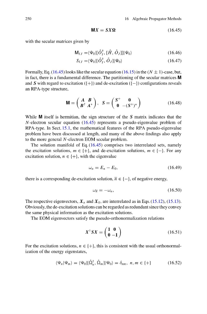
Formally, Eq. (16.45) looks like the secular equation (16.15) in the (N ± 1)-case, but,
in fact, there is a fundamental difference. The partitioning of the secular matrices M
and S with regard to excitation ({+}) and de-excitation ({−}) configurations reveals
an RPA-type structure,
M =
A B
B
† A
∗
, S =
S
+
0
0 −(S
+
)
∗
(16.48)
While M itself is hermitian, the sign structure of the S matrix indicates that the
N -electron secular equation (16.45) represents a pseudo-eigenvalue problem of
RPA-type. In Sect. 15.1, the mathematical features of the RPA pseudo-eigenvalue
problem have been discussed at length, and many of the above findings also apply
to the more general N -electron EOM secular problem.
The solution manifold of Eq. (16.45) comprises two interrelated sets, namely
the excitation solutions, m ∈ {+}, and de-excitation solutions, m ∈ {−}. For any
excitation solution, n ∈ {+}, with the eigenvalue
ω n = E n − E 0 ,
(16.49)
there is a corresponding de-excitation solution, n ∈ {−}, of negative energy,
ω n = −ω n ,
(16.50)
The respective eigenvectors, X n and X n , are interrelated as in Eqs. (15.12), (15.13).
Obviously, the de-excitation solutions can be regarded as redundant since they convey
the same physical information as the excitation solutions.
The EOM eigenvectors satisfy the pseudo-orthonormalization relations
X
† SX =
1 0
0 −1
(16.51)
For the excitation solutions, n ∈ {+}, this is consistent with the usual orthonormalization of the energy eigenstates,
n | m = = 0 |[ ˆ
†
n , ˆ
m ]| 0 = δ nm , n, m ∈ {+}
(16.52)
16 Algebraic Propagator Methods
MX = SX
(16.45)
with the secular matrices given by
M I J == 0 |[ ˆ
O
†
I , [ ˆ
H , ˆ
O J ]]| 0
(16.46)
S I J == 0 |[ ˆ
O
†
I , ˆ
O J ]| 0
(16.47)
Formally, Eq. (16.45) looks like the secular equation (16.15) in the (N ± 1)-case, but,
in fact, there is a fundamental difference. The partitioning of the secular matrices M
and S with regard to excitation ({+}) and de-excitation ({−}) configurations reveals
an RPA-type structure,
M =
A B
B
† A
∗
, S =
S
+
0
0 −(S
+
)
∗
(16.48)
While M itself is hermitian, the sign structure of the S matrix indicates that the
N -electron secular equation (16.45) represents a pseudo-eigenvalue problem of
RPA-type. In Sect. 15.1, the mathematical features of the RPA pseudo-eigenvalue
problem have been discussed at length, and many of the above findings also apply
to the more general N -electron EOM secular problem.
The solution manifold of Eq. (16.45) comprises two interrelated sets, namely
the excitation solutions, m ∈ {+}, and de-excitation solutions, m ∈ {−}. For any
excitation solution, n ∈ {+}, with the eigenvalue
ω n = E n − E 0 ,
(16.49)
there is a corresponding de-excitation solution, n ∈ {−}, of negative energy,
ω n = −ω n ,
(16.50)
The respective eigenvectors, X n and X n , are interrelated as in Eqs. (15.12), (15.13).
Obviously, the de-excitation solutions can be regarded as redundant since they convey
the same physical information as the excitation solutions.
The EOM eigenvectors satisfy the pseudo-orthonormalization relations
X
† SX =
1 0
0 −1
(16.51)
For the excitation solutions, n ∈ {+}, this is consistent with the usual orthonormalization of the energy eigenstates,
n | m = = 0 |[ ˆ
†
n , ˆ
m ]| 0 = δ nm , n, m ∈ {+}
(16.52)