

244
16 Algebraic Propagator Methods
will expect that the set of EOM solutions comprises also the energy eigenstates of
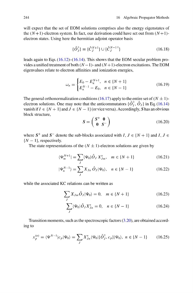
the (N +1)-electron system. In fact, our derivation could have set out from (N +1)electron states. Using here the hermitian adjoint operator basis
{ ˆ
O
†
J } ≡ { ˆ
C
N +1
J
} ∪ { ˆ
C
N −1 †
J
}
(16.18)
leads again to Eqs. (16.12)–(16.14). This shows that the EOM secular problem provides a unified treatment of both (N −1)- and (N +1)-electron excitations. The EOM
eigenvalues relate to electron affinities and ionization energies,
ω n =
E 0 − E
N +1
n
, n ∈ {N + 1}
E
N −1
n
− E 0 , n ∈ {N − 1}
(16.19)
The general orthonormalization conditions (16.17) apply to the entire set of (N ± 1)electron solutions. One may note that the anticommutators { ˆ
O
†
I , ˆ
O J } in Eq. (16.14)
vanish if I ∈ {N + 1} and J ∈ {N − 1} (or vice versa). Accordingly, S has an obvious
block structure,
S =
S
+ 0
0 S
−
(16.20)
where S
+ and S
− denote the sub-blocks associated with I, J ∈ {N + 1} and I, J ∈
{N − 1}, respectively.
The state representations of the (N ± 1)-electron solutions are given by
N +1
m
| =
J
0 | ˆ
O J X
∗
J m , m ∈ {N + 1}
(16.21)
|
N −1
n
=
J
X J n ˆ
O J | 0 , n ∈ {N − 1}
(16.22)
while the associated KC relations can be written as
J
X J m ˆ
O J | 0 = 0, m ∈ {N + 1}
(16.23)
J
0 | ˆ
O J X
∗
J n = 0, n ∈ {N − 1}
(16.24)
Transition moments, such as the spectroscopic factors (3.20), are obtained according to
x
(n)
p = =
N −1
|c p | 0 =
J
X
∗
J n 0 |{ ˆ
O
†
J , c p }| 0 , n ∈ {N − 1}
(16.25)
16 Algebraic Propagator Methods
will expect that the set of EOM solutions comprises also the energy eigenstates of
the (N +1)-electron system. In fact, our derivation could have set out from (N +1)electron states. Using here the hermitian adjoint operator basis
{ ˆ
O
†
J } ≡ { ˆ
C
N +1
J
} ∪ { ˆ
C
N −1 †
J
}
(16.18)
leads again to Eqs. (16.12)–(16.14). This shows that the EOM secular problem provides a unified treatment of both (N −1)- and (N +1)-electron excitations. The EOM
eigenvalues relate to electron affinities and ionization energies,
ω n =
E 0 − E
N +1
n
, n ∈ {N + 1}
E
N −1
n
− E 0 , n ∈ {N − 1}
(16.19)
The general orthonormalization conditions (16.17) apply to the entire set of (N ± 1)electron solutions. One may note that the anticommutators { ˆ
O
†
I , ˆ
O J } in Eq. (16.14)
vanish if I ∈ {N + 1} and J ∈ {N − 1} (or vice versa). Accordingly, S has an obvious
block structure,
S =
S
+ 0
0 S
−
(16.20)
where S
+ and S
− denote the sub-blocks associated with I, J ∈ {N + 1} and I, J ∈
{N − 1}, respectively.
The state representations of the (N ± 1)-electron solutions are given by
N +1
m
| =
J
0 | ˆ
O J X
∗
J m , m ∈ {N + 1}
(16.21)
|
N −1
n
=
J
X J n ˆ
O J | 0 , n ∈ {N − 1}
(16.22)
while the associated KC relations can be written as
J
X J m ˆ
O J | 0 = 0, m ∈ {N + 1}
(16.23)
J
0 | ˆ
O J X
∗
J n = 0, n ∈ {N − 1}
(16.24)
Transition moments, such as the spectroscopic factors (3.20), are obtained according to
x
(n)
p = =
N −1
|c p | 0 =
J
X
∗
J n 0 |{ ˆ
O
†
J , c p }| 0 , n ∈ {N − 1}
(16.25)