

228
15 Random-Phase Approximation (RPA)
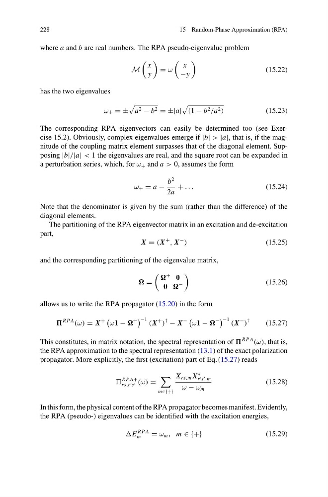
where a and b are real numbers. The RPA pseudo-eigenvalue problem
M
x
y
= ω
x
−y
(15.22)
has the two eigenvalues
ω ± = ±
a 2 − b 2 = ±|a|
(1 − b 2 /a 2 )
(15.23)
The corresponding RPA eigenvectors can easily be determined too (see Exercise 15.2). Obviously, complex eigenvalues emerge if |b| > |a|, that is, if the magnitude of the coupling matrix element surpasses that of the diagonal element. Supposing |b|/|a| < 1 the eigenvalues are real, and the square root can be expanded in
a perturbation series, which, for ω + and a > 0, assumes the form
ω + = a −
b
2
2a
+ . . .
(15.24)
Note that the denominator is given by the sum (rather than the difference) of the
diagonal elements.
The partitioning of the RPA eigenvector matrix in an excitation and de-excitation
part,
X = (X
+
, X
−
)
(15.25)
and the corresponding partitioning of the eigenvalue matrix,
=
+ 0
0
−
(15.26)
allows us to write the RPA propagator (15.20) in the form
R P A
(ω) = X
+
ω1 −
+
−1 (X
+
)
†
− X
−
ω1 −
−
−1 (X
−
)
†
(15.27)
This constitutes, in matrix notation, the spectral representation of
R P A
(ω), that is,
the RPA approximation to the spectral representation (13.1) of the exact polarization
propagator. More explicitly, the first (excitation) part of Eq. (15.27) reads
R P A+
rs,r s (ω) =
m∈{+}
X rs,m X
∗
r s ,m
ω − ω m
(15.28)
In this form, the physical content of the RPA propagator becomes manifest. Evidently,
the RPA (pseudo-) eigenvalues can be identified with the excitation energies,
E
R P A
m
= ω m , m ∈ {+}
(15.29)
15 Random-Phase Approximation (RPA)
where a and b are real numbers. The RPA pseudo-eigenvalue problem
M
x
y
= ω
x
−y
(15.22)
has the two eigenvalues
ω ± = ±
a 2 − b 2 = ±|a|
(1 − b 2 /a 2 )
(15.23)
The corresponding RPA eigenvectors can easily be determined too (see Exercise 15.2). Obviously, complex eigenvalues emerge if |b| > |a|, that is, if the magnitude of the coupling matrix element surpasses that of the diagonal element. Supposing |b|/|a| < 1 the eigenvalues are real, and the square root can be expanded in
a perturbation series, which, for ω + and a > 0, assumes the form
ω + = a −
b
2
2a
+ . . .
(15.24)
Note that the denominator is given by the sum (rather than the difference) of the
diagonal elements.
The partitioning of the RPA eigenvector matrix in an excitation and de-excitation
part,
X = (X
+
, X
−
)
(15.25)
and the corresponding partitioning of the eigenvalue matrix,
=
+ 0
0
−
(15.26)
allows us to write the RPA propagator (15.20) in the form
R P A
(ω) = X
+
ω1 −
+
−1 (X
+
)
†
− X
−
ω1 −
−
−1 (X
−
)
†
(15.27)
This constitutes, in matrix notation, the spectral representation of
R P A
(ω), that is,
the RPA approximation to the spectral representation (13.1) of the exact polarization
propagator. More explicitly, the first (excitation) part of Eq. (15.27) reads
R P A+
rs,r s (ω) =
m∈{+}
X rs,m X
∗
r s ,m
ω − ω m
(15.28)
In this form, the physical content of the RPA propagator becomes manifest. Evidently,
the RPA (pseudo-) eigenvalues can be identified with the excitation energies,
E
R P A
m
= ω m , m ∈ {+}
(15.29)