

186
12 Order Relations and Separability
D AA
0
D A,AB
0
D BB
D B,AB
D AB,A D AB,B
D AB,AB
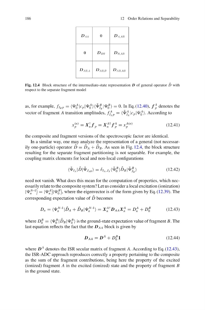
Fig. 12.4 Block structure of the intermediate-state representation D of general operator ˆ
D with
respect to the separate fragment model
as, for example, f I B p = =
A
0 |c p |
A
0 ˜
B
I B
|
B
0 = 0. In Eq. (12.40), f
A
p denotes the
vector of fragment A transition amplitudes, f
A
I A p = = ˜
A
I A
|c p |
A
0 . According to
x
(n)
p = X
†
n f p = X
A†
n f
A
p = x
A(n)
p
(12.41)
the composite and fragment versions of the spectroscopic factor are identical.
In a similar way, one may analyze the representation of a general (not necessarily one-particle) operator ˆ
D = ˆ
D A + ˆ
D B . As seen in Fig. 12.4, the block structure
resulting for the separate fragment partitioning is not separable. For example, the
coupling matrix elements for local and non-local configurations
˜
I A | ˆ
D| ˜
J AB = δ I A ,J A ˜
B
0 | ˆ
D B | ˜
B
J B
(12.42)
need not vanish. What does this mean for the computation of properties, which necessarily relate to the composite system? Let us consider a local excitation (ionization)
|
N−1
n
= |
A
n
|
B
0
, where the eigenvector is of the form given by Eq. (12.39). The
corresponding expectation value of ˆ
D becomes
D n = =
N−1
n | ˆ
D A + ˆ
D B |
N−1
n = X
A†
n D A A X
A
n = D
A
n + D
B
0
(12.43)
where D
B
0 = =
B
0 | ˆ
D B |
B
0 is the ground-state expectation value of fragment B. The
last equation reflects the fact that the D A A block is given by
D A A = D
A
+ D
B
0 1
(12.44)
where D
A denotes the ISR secular matrix of fragment A. According to Eq. (12.43),
the ISR-ADC approach reproduces correctly a property pertaining to the composite
as the sum of the fragment contributions, being here the property of the excited
(ionized) fragment A in the excited (ionized) state and the property of fragment B
in the ground state.
12 Order Relations and Separability
D AA
0
D A,AB
0
D BB
D B,AB
D AB,A D AB,B
D AB,AB
Fig. 12.4 Block structure of the intermediate-state representation D of general operator ˆ
D with
respect to the separate fragment model
as, for example, f I B p = =
A
0 |c p |
A
0 ˜
B
I B
|
B
0 = 0. In Eq. (12.40), f
A
p denotes the
vector of fragment A transition amplitudes, f
A
I A p = = ˜
A
I A
|c p |
A
0 . According to
x
(n)
p = X
†
n f p = X
A†
n f
A
p = x
A(n)
p
(12.41)
the composite and fragment versions of the spectroscopic factor are identical.
In a similar way, one may analyze the representation of a general (not necessarily one-particle) operator ˆ
D = ˆ
D A + ˆ
D B . As seen in Fig. 12.4, the block structure
resulting for the separate fragment partitioning is not separable. For example, the
coupling matrix elements for local and non-local configurations
˜
I A | ˆ
D| ˜
J AB = δ I A ,J A ˜
B
0 | ˆ
D B | ˜
B
J B
(12.42)
need not vanish. What does this mean for the computation of properties, which necessarily relate to the composite system? Let us consider a local excitation (ionization)
|
N−1
n
= |
A
n
|
B
0
, where the eigenvector is of the form given by Eq. (12.39). The
corresponding expectation value of ˆ
D becomes
D n = =
N−1
n | ˆ
D A + ˆ
D B |
N−1
n = X
A†
n D A A X
A
n = D
A
n + D
B
0
(12.43)
where D
B
0 = =
B
0 | ˆ
D B |
B
0 is the ground-state expectation value of fragment B. The
last equation reflects the fact that the D A A block is given by
D A A = D
A
+ D
B
0 1
(12.44)
where D
A denotes the ISR secular matrix of fragment A. According to Eq. (12.43),
the ISR-ADC approach reproduces correctly a property pertaining to the composite
as the sum of the fragment contributions, being here the property of the excited
(ionized) fragment A in the excited (ionized) state and the property of fragment B
in the ground state.