

11.3 Intermediate-State Representation of General Operators
173
D 0 (2) = D
(0)
0 + D
(2)
0 + O(3)
(11.66)
extends through second order, whereas in ˜
D 22 only the zeroth-order term
D
(0)
0 = = 0 | ˆ
D| 0 =
j
d j j
(11.67)
is needed. Note that D
(1)
0 = 0.
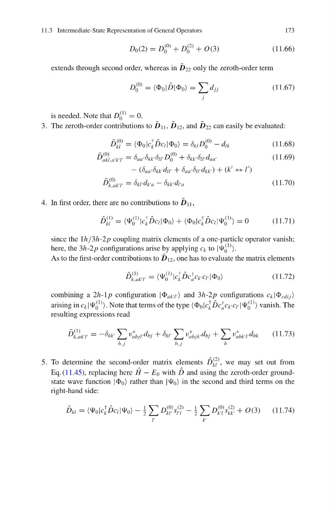
3. The zeroth-order contributions to ˜
D 11 , ˜
D 12 , and ˜
D 22 can easily be evaluated:
˜
D
(0)
kl = = 0 |c
†
k
ˆ
Dc l | 0 = δ kl D
(0)
0 − d lk
(11.68)
˜
D
(0)
akl,a k l = δ aa δ kk δ ll D
(0)
0 + δ kk δ ll d aa
(11.69)
− (δ aa δ kk d ll + δ aa δ ll d kk ) + (k
↔ l
)
˜
D
(0)
k,ak l = δ kl d k a − δ kk d l a
(11.70)
4. In first order, there are no contributions to ˜
D 11 ,
˜
D
(1)
kl = =
(1)
0 |c
†
k
ˆ
Dc l | 0 + + 0 |c
†
k
ˆ
Dc l |
(1)
0 = 0
(11.71)
since the 1h/3h-2 p coupling matrix elements of a one-particle operator vanish;
here, the 3h-2 p configurations arise by applying c k to |
(1)
0 .
As to the first-order contributions to ˜
D 12 , one has to evaluate the matrix elements
˜
D
(1)
k,ak l = =
(1)
0 |c
†
k
ˆ
Dc
†
a c k c l | 0
(11.72)
combining a 2h-1 p configuration | ak l and 3h-2 p configurations c k | cdi j
arising in c k |
(1)
0 . Note that terms of the type 0 |c
†
k
ˆ
Dc
†
a c k c l |
(1)
0 vanish. The
resulting expressions read
˜
D
(1)
k,ak l = −δ kk
b, j
v
∗
abjl d bj + δ kl
b, j
v
∗
abjk d bj +
b
v
∗
abk l d bk
(11.73)
5. To determine the second-order matrix elements ˜
D
(2)
kl , we may set out from
Eq. (11.45), replacing here ˆ
H − E 0 with ˆ
D and using the zeroth-order groundstate wave function | 0 rather than | 0 in the second and third terms on the
right-hand side:
˜
D kl = = 0 |c
†
k
ˆ
Dc l | 0 −
1
2
l
D
(0)
kl s
(2)
l l −
1
2
k
D
(0)
k l s
(2)
kk + O(3)
(11.74)
173
D 0 (2) = D
(0)
0 + D
(2)
0 + O(3)
(11.66)
extends through second order, whereas in ˜
D 22 only the zeroth-order term
D
(0)
0 = = 0 | ˆ
D| 0 =
j
d j j
(11.67)
is needed. Note that D
(1)
0 = 0.
3. The zeroth-order contributions to ˜
D 11 , ˜
D 12 , and ˜
D 22 can easily be evaluated:
˜
D
(0)
kl = = 0 |c
†
k
ˆ
Dc l | 0 = δ kl D
(0)
0 − d lk
(11.68)
˜
D
(0)
akl,a k l = δ aa δ kk δ ll D
(0)
0 + δ kk δ ll d aa
(11.69)
− (δ aa δ kk d ll + δ aa δ ll d kk ) + (k
↔ l
)
˜
D
(0)
k,ak l = δ kl d k a − δ kk d l a
(11.70)
4. In first order, there are no contributions to ˜
D 11 ,
˜
D
(1)
kl = =
(1)
0 |c
†
k
ˆ
Dc l | 0 + + 0 |c
†
k
ˆ
Dc l |
(1)
0 = 0
(11.71)
since the 1h/3h-2 p coupling matrix elements of a one-particle operator vanish;
here, the 3h-2 p configurations arise by applying c k to |
(1)
0 .
As to the first-order contributions to ˜
D 12 , one has to evaluate the matrix elements
˜
D
(1)
k,ak l = =
(1)
0 |c
†
k
ˆ
Dc
†
a c k c l | 0
(11.72)
combining a 2h-1 p configuration | ak l and 3h-2 p configurations c k | cdi j
arising in c k |
(1)
0 . Note that terms of the type 0 |c
†
k
ˆ
Dc
†
a c k c l |
(1)
0 vanish. The
resulting expressions read
˜
D
(1)
k,ak l = −δ kk
b, j
v
∗
abjl d bj + δ kl
b, j
v
∗
abjk d bj +
b
v
∗
abk l d bk
(11.73)
5. To determine the second-order matrix elements ˜
D
(2)
kl , we may set out from
Eq. (11.45), replacing here ˆ
H − E 0 with ˆ
D and using the zeroth-order groundstate wave function | 0 rather than | 0 in the second and third terms on the
right-hand side:
˜
D kl = = 0 |c
†
k
ˆ
Dc l | 0 −
1
2
l
D
(0)
kl s
(2)
l l −
1
2
k
D
(0)
k l s
(2)
kk + O(3)
(11.74)