

11.3 Intermediate-State Representation of General Operators
171
D nm = =
N−1
n | ˆ
D|
N−1
m = X
†
n
˜
DX m
(11.53)
As another useful option enabled by the generalization of the ISR, the original
hamiltonian ˆ
H can be easily augmented with an additional (external) operator ˆ
U ,
ˆ
H → ˆ
H
x
= ˆ
H + ˆ
U
(11.54)
The operator ˆ
U may represent any perturbation of the system, such as an external
field. The important point here is that ˆ
U acts on the (N −1)-particle system, but does
not affect the original N -electron ground state. The extended secular equations read
(M + ˜
U)X = X
x
, X
† X = 1
(11.55)
where U is the ISR of the external operator ˆ
U .
In the case of a time-dependent external potential, ˆ
U (t), the time-dependent
Schrödinger equation
i
∂
∂t
|(t) = ( ˆ
H + ˆ
U (t))|(t)
(11.56)
becomes amenable to propagation schemes, such as,
x(t + dt) = x(t) − i(M + ˜
U(t))x(t)dt
(11.57)
based on the IS representation of ˆ
U (t); here, x(t) is the vector of the expansion
coefficients x I (t) = = ˜
I |(t).
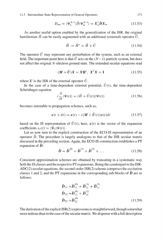
Let us now turn to the explicit construction of the ECO-IS representation of an
operator ˆ
D. The procedure is largely analogous to that of the ISR secular matrix
discussed in the preceding section. Again, the ECO-IS construction establishes a PT
expansion of ˜
D:
˜
D = ˜
D
(0) + ˜
D
(1) + ˜
D
(2) + . . .
(11.58)
Consistent approximation schemes are obtained by truncating in a systematic way
both the IS classes and the respective PT expansions. Being the counterpart to the ISRADC(2) secular equations, the second-order ISR(2) scheme comprises the excitation
classes 1 and 2, and the PT expansions in the corresponding sub-blocks of ˜
D are as
follows:
˜
D 11 = ˜
D
(0)
11 + ˜
D
(1)
11 + ˜
D
(2)
11
˜
D 12 = ˜
D
(0)
12 + ˜
D
(1)
12
˜
D 22 = ˜
D
(0)
22
(11.59)
The derivation of the explicit ISR(2) expressions is straightforward, though somewhat
more tedious than in the case of the secular matrix. We dispense with a full description
171
D nm = =
N−1
n | ˆ
D|
N−1
m = X
†
n
˜
DX m
(11.53)
As another useful option enabled by the generalization of the ISR, the original
hamiltonian ˆ
H can be easily augmented with an additional (external) operator ˆ
U ,
ˆ
H → ˆ
H
x
= ˆ
H + ˆ
U
(11.54)
The operator ˆ
U may represent any perturbation of the system, such as an external
field. The important point here is that ˆ
U acts on the (N −1)-particle system, but does
not affect the original N -electron ground state. The extended secular equations read
(M + ˜
U)X = X
x
, X
† X = 1
(11.55)
where U is the ISR of the external operator ˆ
U .
In the case of a time-dependent external potential, ˆ
U (t), the time-dependent
Schrödinger equation
i
∂
∂t
|(t) = ( ˆ
H + ˆ
U (t))|(t)
(11.56)
becomes amenable to propagation schemes, such as,
x(t + dt) = x(t) − i(M + ˜
U(t))x(t)dt
(11.57)
based on the IS representation of ˆ
U (t); here, x(t) is the vector of the expansion
coefficients x I (t) = = ˜
I |(t).
Let us now turn to the explicit construction of the ECO-IS representation of an
operator ˆ
D. The procedure is largely analogous to that of the ISR secular matrix
discussed in the preceding section. Again, the ECO-IS construction establishes a PT
expansion of ˜
D:
˜
D = ˜
D
(0) + ˜
D
(1) + ˜
D
(2) + . . .
(11.58)
Consistent approximation schemes are obtained by truncating in a systematic way
both the IS classes and the respective PT expansions. Being the counterpart to the ISRADC(2) secular equations, the second-order ISR(2) scheme comprises the excitation
classes 1 and 2, and the PT expansions in the corresponding sub-blocks of ˜
D are as
follows:
˜
D 11 = ˜
D
(0)
11 + ˜
D
(1)
11 + ˜
D
(2)
11
˜
D 12 = ˜
D
(0)
12 + ˜
D
(1)
12
˜
D 22 = ˜
D
(0)
22
(11.59)
The derivation of the explicit ISR(2) expressions is straightforward, though somewhat
more tedious than in the case of the secular matrix. We dispense with a full description