

10.2 Explicit ADC Procedure Through Second Order
151
˜
G
(0)
pq (ω) = δ pq (ω − p )
−1 n p
This shows that all blocks f
(0)
μ vanish except for μ = 1,
f
(0)
μ = 0, for μ > 1
(10.20)
and f
(0)
1 is given by
f
(0)
pq = δ pq n p
(10.21)
First Order:
Since f
(0)
1 is the only non-vanishing zeroth-order block of f , the first-order ADC
form can be written more specifically as
˜
G
(1) (ω) = f
(1)†
1 (ω − K 1 )
−1 f
(0)
1 + h.c.
+ f
(0)†
1 (ω − K 1 )
−1 C
(1)
11 (ω − K 1 )
−1 f
(0)
1
(10.22)
displaying the matrix blocks f
(1)
1 and C
(1)
11 as new constituents. The formal ADC
expression is to be compared to the (vanishing) first-order propagator contribution,
G
(1)−
(ω) = 0, (see Sect. 6.2), which gives
C
(1)
11 = 0
f
(1)
1 = 0
(10.23)
Second Order:
In second order, the ADC expansion takes on the form
˜
G
(2) (ω) = f
(2)
1
† (ω − K 1 )
−1 f
(0)
1 + h.c.
( a)
+ f
(0)
1
† (ω − K 1 )
−1 C
(2)
11 (ω − K 1 )
−1 f
(0)
1
(b)
+ f
(1)
2
† (ω − K 2 )
−1 f
(1)
2 + . . .
(c)
+ f
(0)
1
† (ω − K 1 )
−1 C
(1)
12 (ω − K 2 )
−1 C
(1)
21 (ω − K 1 )
−1 f
(0)
1 + . . . (d)
+ f
(0)
1
† (ω − K 1 )
−1 C
(1)
12 (ω − K 2 )
−1 f
(1)
2 + · · · + h.c.
( e)
(10.24)
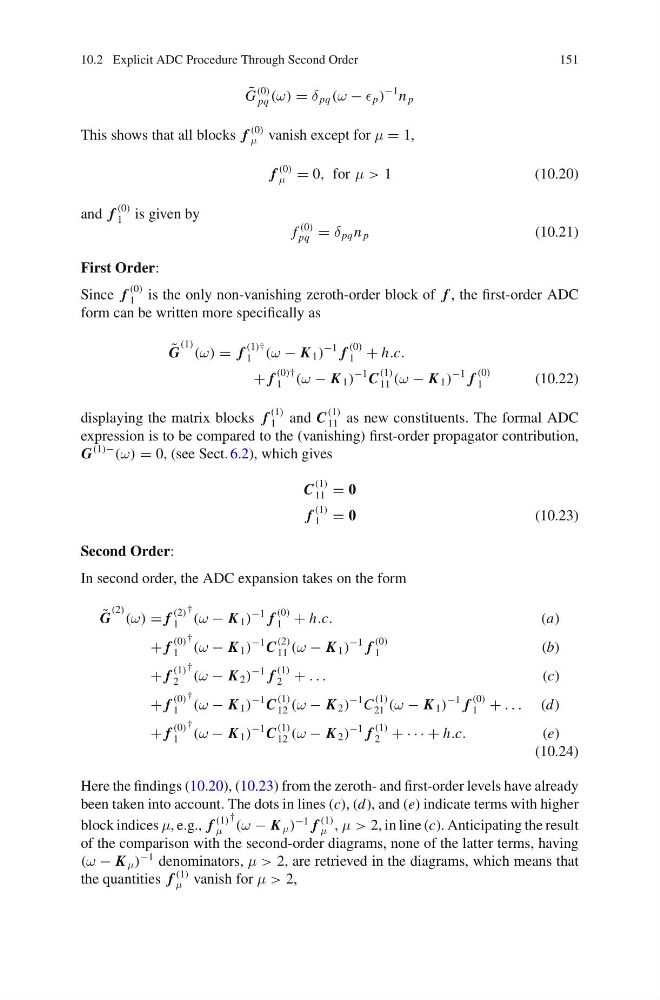
Here the findings (10.20), (10.23) from the zeroth- and first-order levels have already
been taken into account. The dots in lines (c), (d), and (e) indicate terms with higher
block indices μ, e.g., f
(1)
μ
† (ω − K μ )
−1 f
(1)
μ , μ > 2, in line (c). Anticipating the result
of the comparison with the second-order diagrams, none of the latter terms, having
(ω − K μ )
−1 denominators, μ > 2, are retrieved in the diagrams, which means that
the quantities f
(1)
μ vanish for μ > 2,
151
˜
G
(0)
pq (ω) = δ pq (ω − p )
−1 n p
This shows that all blocks f
(0)
μ vanish except for μ = 1,
f
(0)
μ = 0, for μ > 1
(10.20)
and f
(0)
1 is given by
f
(0)
pq = δ pq n p
(10.21)
First Order:
Since f
(0)
1 is the only non-vanishing zeroth-order block of f , the first-order ADC
form can be written more specifically as
˜
G
(1) (ω) = f
(1)†
1 (ω − K 1 )
−1 f
(0)
1 + h.c.
+ f
(0)†
1 (ω − K 1 )
−1 C
(1)
11 (ω − K 1 )
−1 f
(0)
1
(10.22)
displaying the matrix blocks f
(1)
1 and C
(1)
11 as new constituents. The formal ADC
expression is to be compared to the (vanishing) first-order propagator contribution,
G
(1)−
(ω) = 0, (see Sect. 6.2), which gives
C
(1)
11 = 0
f
(1)
1 = 0
(10.23)
Second Order:
In second order, the ADC expansion takes on the form
˜
G
(2) (ω) = f
(2)
1
† (ω − K 1 )
−1 f
(0)
1 + h.c.
( a)
+ f
(0)
1
† (ω − K 1 )
−1 C
(2)
11 (ω − K 1 )
−1 f
(0)
1
(b)
+ f
(1)
2
† (ω − K 2 )
−1 f
(1)
2 + . . .
(c)
+ f
(0)
1
† (ω − K 1 )
−1 C
(1)
12 (ω − K 2 )
−1 C
(1)
21 (ω − K 1 )
−1 f
(0)
1 + . . . (d)
+ f
(0)
1
† (ω − K 1 )
−1 C
(1)
12 (ω − K 2 )
−1 f
(1)
2 + · · · + h.c.
( e)
(10.24)
Here the findings (10.20), (10.23) from the zeroth- and first-order levels have already
been taken into account. The dots in lines (c), (d), and (e) indicate terms with higher
block indices μ, e.g., f
(1)
μ
† (ω − K μ )
−1 f
(1)
μ , μ > 2, in line (c). Anticipating the result
of the comparison with the second-order diagrams, none of the latter terms, having
(ω − K μ )
−1 denominators, μ > 2, are retrieved in the diagrams, which means that
the quantities f
(1)
μ vanish for μ > 2,