

8.3 Solving the Dyson Equation
125
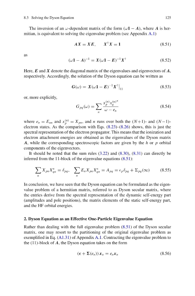
The inversion of an ω-dependent matrix of the form (ω1 − A), where A is hermitian, is equivalent to solving the eigenvalue problem (see Appendix A.1)
AX = X E,
X
† X = 1
(8.51)
as
(ω1 − A)
−1
= X(ω1 − E)
−1 X
†
(8.52)
Here, E and X denote the diagonal matrix of the eigenvalues and eigenvectors of A,
respectively. Accordingly, the solution of the Dyson equation can be written as
G(ω) = X(ω1 − E)
−1 X
†
11
(8.53)
or, more explicitly,
G pq (ω) =
n
x
(n)
p x
(n)
q
∗
ω − e n
(8.54)
where e n = E nn and x
(n)
p = X pn , and n runs over both the (N +1)- and (N −1)electron states. As the comparison with Eqs. (8.23)–(8.26) shows, this is just the
spectral representation of the electron propagator. This means that the ionization and
electron attachment energies are obtained as the eigenvalues of the Dyson matrix
A, while the corresponding spectroscopic factors are given by the h or p orbital
components of the eigenvectors.
It should be noted that the sum rules (3.22) and (8.30), (8.31) can directly be
inferred from the 11-block of the eigenvalue equations (8.51):
n
X pn X
∗
qn = δ pq ,
n
E n X pn X
∗
qn = A pq = p δ pq + pq (∞)
(8.55)
In conclusion, we have seen that the Dyson equation can be formulated as the eigenvalue problem of a hermitian matrix, referred to as Dyson secular matrix, where
the entries derive from the spectral representation of the dynamic self-energy part
(amplitudes and pole positions), the matrix elements of the static self-energy part,
and the HF orbital energies.
2. Dyson Equation as an Effective One-Particle Eigenvalue Equation
Rather than dealing with the full eigenvalue problem (8.51) of the Dyson secular
matrix, one may resort to the partitioning of the original eigenvalue problem as
exemplified in Eq. (A1.31) of Appendix A.1. Contracting the eigenvalue problem to
the (11)-block of A, the Dyson equation takes on the form
( + (e n )) x n = e n x n
(8.56)
125
The inversion of an ω-dependent matrix of the form (ω1 − A), where A is hermitian, is equivalent to solving the eigenvalue problem (see Appendix A.1)
AX = X E,
X
† X = 1
(8.51)
as
(ω1 − A)
−1
= X(ω1 − E)
−1 X
†
(8.52)
Here, E and X denote the diagonal matrix of the eigenvalues and eigenvectors of A,
respectively. Accordingly, the solution of the Dyson equation can be written as
G(ω) = X(ω1 − E)
−1 X
†
11
(8.53)
or, more explicitly,
G pq (ω) =
n
x
(n)
p x
(n)
q
∗
ω − e n
(8.54)
where e n = E nn and x
(n)
p = X pn , and n runs over both the (N +1)- and (N −1)electron states. As the comparison with Eqs. (8.23)–(8.26) shows, this is just the
spectral representation of the electron propagator. This means that the ionization and
electron attachment energies are obtained as the eigenvalues of the Dyson matrix
A, while the corresponding spectroscopic factors are given by the h or p orbital
components of the eigenvectors.
It should be noted that the sum rules (3.22) and (8.30), (8.31) can directly be
inferred from the 11-block of the eigenvalue equations (8.51):
n
X pn X
∗
qn = δ pq ,
n
E n X pn X
∗
qn = A pq = p δ pq + pq (∞)
(8.55)
In conclusion, we have seen that the Dyson equation can be formulated as the eigenvalue problem of a hermitian matrix, referred to as Dyson secular matrix, where
the entries derive from the spectral representation of the dynamic self-energy part
(amplitudes and pole positions), the matrix elements of the static self-energy part,
and the HF orbital energies.
2. Dyson Equation as an Effective One-Particle Eigenvalue Equation
Rather than dealing with the full eigenvalue problem (8.51) of the Dyson secular
matrix, one may resort to the partitioning of the original eigenvalue problem as
exemplified in Eq. (A1.31) of Appendix A.1. Contracting the eigenvalue problem to
the (11)-block of A, the Dyson equation takes on the form
( + (e n )) x n = e n x n
(8.56)