

112
8 Self-Energy and the Dyson Equation
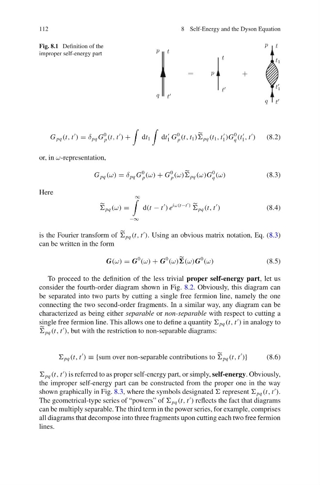
Fig. 8.1 Definition of the
improper self-energy part
G pq (t, t
) = δ pq G
0
p (t, t
) +
dt 1
dt
1 G
0
p (t, t 1 )
pq (t 1 , t
1 )G
0
q (t
1 , t
)
(8.2)
or, in ω-representation,
G pq (ω) = δ pq G
0
p (ω) + G
0
p (ω)
pq (ω)G
0
q (ω)
(8.3)
Here
pq (ω) =
∞
−∞
d(t − t
) e
iω(t−t
)
pq (t, t
)
(8.4)
is the Fourier transform of
pq (t, t
). Using an obvious matrix notation, Eq. (8.3)
can be written in the form
G(ω) = G
0
(ω) + G
0
(ω)
(ω)G
0
(ω)
(8.5)
To proceed to the definition of the less trivial proper self-energy part, let us
consider the fourth-order diagram shown in Fig. 8.2. Obviously, this diagram can
be separated into two parts by cutting a single free fermion line, namely the one
connecting the two second-order fragments. In a similar way, any diagram can be
characterized as being either separable or non-separable with respect to cutting a
single free fermion line. This allows one to define a quantity pq (t, t
) in analogy to
pq (t, t
), but with the restriction to non-separable diagrams:
pq (t, t
) ≡ {sum over non-separable contributions to
pq (t, t
)}
(8.6)
pq (t, t
) is referred to as proper self-energy part, or simply, self-energy. Obviously,
the improper self-energy part can be constructed from the proper one in the way
shown graphically in Fig. 8.3, where the symbols designated represent pq (t, t
).
The geometrical-type series of “powers” of pq (t, t
) reflects the fact that diagrams
can be multiply separable. The third term in the power series, for example, comprises
all diagrams that decompose into three fragments upon cutting each two free fermion
lines.
8 Self-Energy and the Dyson Equation
Fig. 8.1 Definition of the
improper self-energy part
G pq (t, t
) = δ pq G
0
p (t, t
) +
dt 1
dt
1 G
0
p (t, t 1 )
pq (t 1 , t
1 )G
0
q (t
1 , t
)
(8.2)
or, in ω-representation,
G pq (ω) = δ pq G
0
p (ω) + G
0
p (ω)
pq (ω)G
0
q (ω)
(8.3)
Here
pq (ω) =
∞
−∞
d(t − t
) e
iω(t−t
)
pq (t, t
)
(8.4)
is the Fourier transform of
pq (t, t
). Using an obvious matrix notation, Eq. (8.3)
can be written in the form
G(ω) = G
0
(ω) + G
0
(ω)
(ω)G
0
(ω)
(8.5)
To proceed to the definition of the less trivial proper self-energy part, let us
consider the fourth-order diagram shown in Fig. 8.2. Obviously, this diagram can
be separated into two parts by cutting a single free fermion line, namely the one
connecting the two second-order fragments. In a similar way, any diagram can be
characterized as being either separable or non-separable with respect to cutting a
single free fermion line. This allows one to define a quantity pq (t, t
) in analogy to
pq (t, t
), but with the restriction to non-separable diagrams:
pq (t, t
) ≡ {sum over non-separable contributions to
pq (t, t
)}
(8.6)
pq (t, t
) is referred to as proper self-energy part, or simply, self-energy. Obviously,
the improper self-energy part can be constructed from the proper one in the way
shown graphically in Fig. 8.3, where the symbols designated represent pq (t, t
).
The geometrical-type series of “powers” of pq (t, t
) reflects the fact that diagrams
can be multiply separable. The third term in the power series, for example, comprises
all diagrams that decompose into three fragments upon cutting each two free fermion
lines.