

104
7 Time-Ordered or Goldstone Diagrams
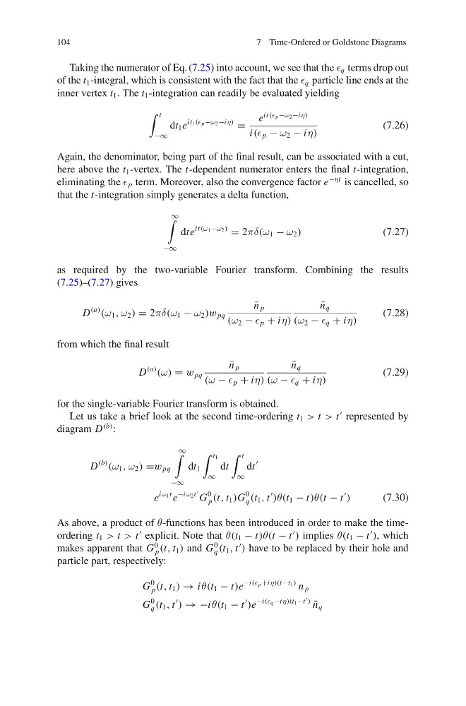
Taking the numerator of Eq. (7.25) into account, we see that the q terms drop out
of the t 1 -integral, which is consistent with the fact that the q particle line ends at the
inner vertex t 1 . The t 1 -integration can readily be evaluated yielding
t
−∞
dt 1 e
it 1 ( p −ω 2 −iη)
=
e
it ( p −ω 2 −iη)
i( p − ω 2 − iη)
(7.26)
Again, the denominator, being part of the final result, can be associated with a cut,
here above the t 1 -vertex. The t-dependent numerator enters the final t-integration,
eliminating the p term. Moreover, also the convergence factor e
−ηt is cancelled, so
that the t-integration simply generates a delta function,
∞
−∞
dte
it (ω 1 −ω 2 )
= 2πδ(ω 1 − ω 2 )
(7.27)
as required by the two-variable Fourier transform. Combining the results
(7.25)–(7.27) gives
D
(a)
(ω 1 , ω 2 ) = 2πδ(ω 1 − ω 2 )w pq
¯
n p
(ω 2 − p + iη)
¯
n q
(ω 2 − q + iη)
(7.28)
from which the final result
D
(a)
(ω) = w pq
¯
n p
(ω − p + iη)
¯
n q
(ω − q + iη)
(7.29)
for the single-variable Fourier transform is obtained.
Let us take a brief look at the second time-ordering t 1 > t > t
represented by
diagram D
(b) :
D
(b)
(ω 1 , ω 2 ) =w pq
∞
−∞
dt 1
t 1
∞
dt
t
∞
dt
e
iω 1 t e
−iω 2 t
G
0
p (t, t 1 )G
0
q (t 1 , t
)θ(t 1 − t)θ(t − t
)
(7.30)
As above, a product of θ-functions has been introduced in order to make the timeordering t 1 > t > t
explicit. Note that θ(t 1 − t)θ(t − t
) implies θ(t 1 − t
), which
makes apparent that G
0
p (t, t 1 ) and G
0
q (t 1 , t
) have to be replaced by their hole and
particle part, respectively:
G
0
p (t, t 1 ) → iθ(t 1 − t)e
−i( p +iη)(t−t 1 ) n p
G
0
q (t 1 , t
) → −iθ(t 1 − t
)e
−i( q −iη)(t 1 −t
)
¯
n q
7 Time-Ordered or Goldstone Diagrams
Taking the numerator of Eq. (7.25) into account, we see that the q terms drop out
of the t 1 -integral, which is consistent with the fact that the q particle line ends at the
inner vertex t 1 . The t 1 -integration can readily be evaluated yielding
t
−∞
dt 1 e
it 1 ( p −ω 2 −iη)
=
e
it ( p −ω 2 −iη)
i( p − ω 2 − iη)
(7.26)
Again, the denominator, being part of the final result, can be associated with a cut,
here above the t 1 -vertex. The t-dependent numerator enters the final t-integration,
eliminating the p term. Moreover, also the convergence factor e
−ηt is cancelled, so
that the t-integration simply generates a delta function,
∞
−∞
dte
it (ω 1 −ω 2 )
= 2πδ(ω 1 − ω 2 )
(7.27)
as required by the two-variable Fourier transform. Combining the results
(7.25)–(7.27) gives
D
(a)
(ω 1 , ω 2 ) = 2πδ(ω 1 − ω 2 )w pq
¯
n p
(ω 2 − p + iη)
¯
n q
(ω 2 − q + iη)
(7.28)
from which the final result
D
(a)
(ω) = w pq
¯
n p
(ω − p + iη)
¯
n q
(ω − q + iη)
(7.29)
for the single-variable Fourier transform is obtained.
Let us take a brief look at the second time-ordering t 1 > t > t
represented by
diagram D
(b) :
D
(b)
(ω 1 , ω 2 ) =w pq
∞
−∞
dt 1
t 1
∞
dt
t
∞
dt
e
iω 1 t e
−iω 2 t
G
0
p (t, t 1 )G
0
q (t 1 , t
)θ(t 1 − t)θ(t − t
)
(7.30)
As above, a product of θ-functions has been introduced in order to make the timeordering t 1 > t > t
explicit. Note that θ(t 1 − t)θ(t − t
) implies θ(t 1 − t
), which
makes apparent that G
0
p (t, t 1 ) and G
0
q (t 1 , t
) have to be replaced by their hole and
particle part, respectively:
G
0
p (t, t 1 ) → iθ(t 1 − t)e
−i( p +iη)(t−t 1 ) n p
G
0
q (t 1 , t
) → −iθ(t 1 − t
)e
−i( q −iη)(t 1 −t
)
¯
n q