

10-3 “Increased-Valence” Theory and Configuration Interaction for N2O4
135
1
2
2
1
1
3
1
3
{(1
)
( – ) } / {(1
) (1 )}
x
y
(17)
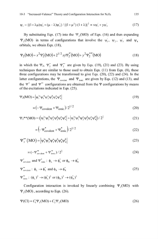
By substituting Eqn. (17) into the 2 (MO)
of Eqn. (16) and then expanding
2 (MO)
in terms of configurations that involve the 1
, 2
, 3
and 4
orbitals, we obtain Eqn. (18),
MO
MO
2
MO
MO
**'
2
2
*'
2
2
/
1
2
2
2
y
xy
x
(18)
in which the ,
*
2
and
**
2
are given by Eqs. (19), (21) and (23). By using
techniques that are similar to those used to obtain Eqn. (11) from Eqn. (8), these
three configurations may be transformed to give Eqs. (20), (22) and (24). In the
latter configurations, the covalent
and ionic
are given by Eqs. (12) and (13), and
the
*
and
**
configurations are obtained from the Ψ configurations by means
of the excitations indicated in Eqn. (25).
2
1
1
2
2 4
4
y (MO)
(19)
2
/
1
ionic
covalent
2
/
(20)
**
1
2
2
1
3
2 2 4 4
3
1
2 2 4 4
(MO) (
) / 2
(21)
2
/
1
*
ionic
*
covalent
2
/
(22)
**'
'α 'β α β α β
2
3 3 2 2 4 4
MO
ψ ψ ψ ψ ψ ψ
(23)
1
2
**
**
cov alent
ionic
(
) / 2
(24)
*
*
*
*
cov alent
ionic
L
L
R
R
and
:
or
**
*
*
cov alent
L
L
R
R
:
and
(25)
**
2
* 2
2
* 2
ionic
L
L
R
R
: ( )
( ) or ( )
( )
Configuration interaction is invoked by linearly combining 1 (MO)
with
2 (MO)
, according to Eqn. (26).
1 1
2
2
(CI)
(MO)
(MO)
C
C
(26)
135
1
2
2
1
1
3
1
3
{(1
)
( – ) } / {(1
) (1 )}
x
y
(17)
By substituting Eqn. (17) into the 2 (MO)
of Eqn. (16) and then expanding
2 (MO)
in terms of configurations that involve the 1
, 2
, 3
and 4
orbitals, we obtain Eqn. (18),
MO
MO
2
MO
MO
**'
2
2
*'
2
2
/
1
2
2
2
y
xy
x
(18)
in which the ,
*
2
and
**
2
are given by Eqs. (19), (21) and (23). By using
techniques that are similar to those used to obtain Eqn. (11) from Eqn. (8), these
three configurations may be transformed to give Eqs. (20), (22) and (24). In the
latter configurations, the covalent
and ionic
are given by Eqs. (12) and (13), and
the
*
and
**
configurations are obtained from the Ψ configurations by means
of the excitations indicated in Eqn. (25).
2
1
1
2
2 4
4
y (MO)
(19)
2
/
1
ionic
covalent
2
/
(20)
**
1
2
2
1
3
2 2 4 4
3
1
2 2 4 4
(MO) (
) / 2
(21)
2
/
1
*
ionic
*
covalent
2
/
(22)
**'
'α 'β α β α β
2
3 3 2 2 4 4
MO
ψ ψ ψ ψ ψ ψ
(23)
1
2
**
**
cov alent
ionic
(
) / 2
(24)
*
*
*
*
cov alent
ionic
L
L
R
R
and
:
or
**
*
*
cov alent
L
L
R
R
:
and
(25)
**
2
* 2
2
* 2
ionic
L
L
R
R
: ( )
( ) or ( )
( )
Configuration interaction is invoked by linearly combining 1 (MO)
with
2 (MO)
, according to Eqn. (26).
1 1
2
2
(CI)
(MO)
(MO)
C
C
(26)