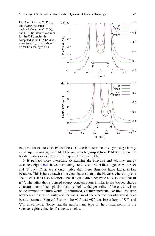
the position of the C–H BCPs (the C–C one is determined by symmetry) hardly
varies upon changing the field. This can better be grasped from Table 6.1, where the
bonded radius of the C atom is displayed for our fields.
It is perhaps more interesting to examine the effective and additive energy
densities. Figure 6.6 shows them along the C–C and C–H lines together with K r
ð Þ
and r
2
q r
ð Þ. First, we should notice that these densities have laplacian-like
behavior. This is here a much more clear feature than in the H 2 case, where only one
shell exists. It is also notorious that the qualitative behavior of K follows that of
E
add . The latter shows bonded energy concentrations similar to the bonded charge
concentrations of the laplacian field. As before, the generality of these results is to
be determined in future works. If confirmed, another energetic-like link, this time
between an energy density and the laplacian of the electron density would have
been uncovered. Figure 6.7 shows the −1.5 and −0.5 a.u. isosurfaces of E
add and
r
2
q in ethylene. Notice that the number and type of the critical points in the
valence region coincides for the two fields.
-1
0
1
2
3
4
5
-4.0
-2.0
0.0
2.0
4.0
0.0
0.2
0.4
0.6
0.8
1.0
Scalar field (a.u.)
x (bohr)
(a)
C
C
ρ
V mep
V xc
-V PAEM
-1
0
1
2
3
4
5
-1.0
0.0
1.0
2.0
3.0
4.0
0.0
0.2
0.4
0.6
0.8
1.0
Scalar field (a.u.)
x (bohr)
(b)
C
H
ρ
V mep
V xc
-V PAEM
Fig. 6.4 Density, MEP, xc,
and PAEM potentials
depicted along the C–C (a),
and C–H (b) internuclear lines
for the C 2 H 4 molecule
computed at the HF//TZV(3d,
p)++ level. V xc and q should
be read on the right axis
6 Emergent Scalar and Vector Fields in Quantum Chemical Topology
143