

68
R. de Nalda et al.
on the image, can be measured by the distance to the center of the image, r. For
the analysis of the kinetic energy distribution (ignoring the angular character), integration over the 2π angular range of the images is carried out. The signal S(v, t),
depending on speed (v) and time (t), is assumed to be composed of individual contributions C i (v, t), each of which has its own temporal shape as a function of time,
i(t), and speed distribution, R i (v). However, C i (v, t) does not need to be separable,
in the sense that some of the parameters of R i (v) may be allowed to depend on time.
It is assumed, in general, that these contributions do not interfere with each other,
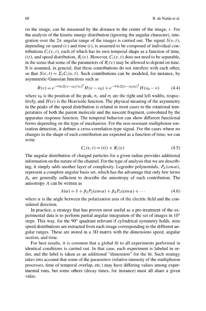
so that S(v, t) = Σ i C i (v, t). Such contributions can be modeled, for instance, by
asymmetric-Gaussian functions such as
R(v) = e
−4 ln 2[(v−v 0 )/σ r ] 2
H (v − v 0 ) + e
−4 ln 2[(v−v 0 )σ l ] 2
H (v 0 − v)
(4.4)
where v 0 is the position of the peak, σ r and σ l are the right and left widths, respectively, and H (v) is the Heaviside function. The physical meaning of the asymmetry
in the peaks of the speed distribution is related in most cases to the rotational temperatures of both the parent molecule and the nascent fragment, convoluted by the
apparatus response function. The temporal behavior can show different functional
forms depending on the type of mechanism. For the non-resonant multiphoton ionization detection, it defines a cross-correlation-type signal. For the cases where no
changes in the shape of each contribution are expected as a function of time, we can
write
C i (v, t) = i(t) × R i (v)
(4.5)
The angular distribution of charged particles for a given radius provides additional
information on the nature of the channel. For the type of analysis that we are describing, it simply adds another layer of complexity. Legendre polynomials, P n (cos α),
represent a complete angular basis set, which has the advantage that only few terms
β n are generally sufficient to describe the anisotropy of each contribution. The
anisotropy A can be written as
A(α) = 1 + β 2 P 2 (cos α) + β 4 P 4 (cos α) + · · ·
(4.6)
where α is the angle between the polarization axis of the electric field and the considered direction.
In practice, a strategy that has proven most useful as a pre-treatment of the experimental data is to perform partial angular integration of the set of images in 10°
steps. This way, for the 90° quadrant relevant if cylindrical symmetry holds, nine
speed distributions are extracted from each image corresponding to the different angular ranges. These are stored in a 3D matrix with the dimensions speed, angular
section, and time.
For best results, it is common that a global fit to all experiments performed in
identical conditions is carried out. In that case, each experiment is labeled in order, and the label is taken as an additional “dimension” for the fit. Such strategy
takes into account that some of the parameters (relative intensity of the multiphoton
processes, time of temporal overlap, etc.) may have differing values among experimental runs, but some others (decay times, for instance) must all share a given
value.
R. de Nalda et al.
on the image, can be measured by the distance to the center of the image, r. For
the analysis of the kinetic energy distribution (ignoring the angular character), integration over the 2π angular range of the images is carried out. The signal S(v, t),
depending on speed (v) and time (t), is assumed to be composed of individual contributions C i (v, t), each of which has its own temporal shape as a function of time,
i(t), and speed distribution, R i (v). However, C i (v, t) does not need to be separable,
in the sense that some of the parameters of R i (v) may be allowed to depend on time.
It is assumed, in general, that these contributions do not interfere with each other,
so that S(v, t) = Σ i C i (v, t). Such contributions can be modeled, for instance, by
asymmetric-Gaussian functions such as
R(v) = e
−4 ln 2[(v−v 0 )/σ r ] 2
H (v − v 0 ) + e
−4 ln 2[(v−v 0 )σ l ] 2
H (v 0 − v)
(4.4)
where v 0 is the position of the peak, σ r and σ l are the right and left widths, respectively, and H (v) is the Heaviside function. The physical meaning of the asymmetry
in the peaks of the speed distribution is related in most cases to the rotational temperatures of both the parent molecule and the nascent fragment, convoluted by the
apparatus response function. The temporal behavior can show different functional
forms depending on the type of mechanism. For the non-resonant multiphoton ionization detection, it defines a cross-correlation-type signal. For the cases where no
changes in the shape of each contribution are expected as a function of time, we can
write
C i (v, t) = i(t) × R i (v)
(4.5)
The angular distribution of charged particles for a given radius provides additional
information on the nature of the channel. For the type of analysis that we are describing, it simply adds another layer of complexity. Legendre polynomials, P n (cos α),
represent a complete angular basis set, which has the advantage that only few terms
β n are generally sufficient to describe the anisotropy of each contribution. The
anisotropy A can be written as
A(α) = 1 + β 2 P 2 (cos α) + β 4 P 4 (cos α) + · · ·
(4.6)
where α is the angle between the polarization axis of the electric field and the considered direction.
In practice, a strategy that has proven most useful as a pre-treatment of the experimental data is to perform partial angular integration of the set of images in 10°
steps. This way, for the 90° quadrant relevant if cylindrical symmetry holds, nine
speed distributions are extracted from each image corresponding to the different angular ranges. These are stored in a 3D matrix with the dimensions speed, angular
section, and time.
For best results, it is common that a global fit to all experiments performed in
identical conditions is carried out. In that case, each experiment is labeled in order, and the label is taken as an additional “dimension” for the fit. Such strategy
takes into account that some of the parameters (relative intensity of the multiphoton
processes, time of temporal overlap, etc.) may have differing values among experimental runs, but some others (decay times, for instance) must all share a given
value.