

Appendix C: The Dirac δ Function and the Normalization of Continuum States
225
|ψ λ are eigenstates of a normal operator, they are or can be chosen to be orthogonal,
so ˆ
E
ψ j
=
ψ j
as already seen in Appendix B. For a continuum state we have
ˆ
E |ψ λ =
λ max
λ min
|ψ λ ψ λ |ψ λ dλ
(C.12)
Since eigenvectors with different eigenvalues are orthogonal, for λ = λ
we have no
contribution to the integral. If we want this expression to yield |ψ λ , we must require
ψ λ |ψ λ = δ(λ − λ
)
(C.13)
We shall then say that |ψ λ is “normalized to the δ of λ.”
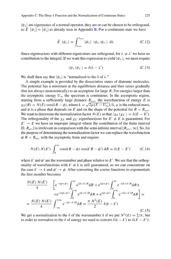
A simple example is provided by the dissociative states of diatomic molecules.
The potential has a minimum at the equilibrium distance and then raises gradually
(but not always monotonically) to an asymptote for large R. For energies larger than
the asymptotic energy U ∞ the spectrum is continuous. In the asymptotic region,
starting from a sufficiently large distance R asy , the wavefunction of energy E is
χ E (R) = N (E) cos(k R − φ), where k =
√
2μ(E − U ∞ )/, μ is the reduced mass,
and φ is a phase that depends on E and on the shape of the potential for R < R asy .
We want to determine the normalization factor N (E) so that χ E |χ E = δ(E − E
).
The orthogonality of the χ E and χ E eigenfunctions for E
= E is guaranteed. For
E
→ E we have an improper integral where the contribution of the finite interval
[0, R asy ] is irrelevant in comparison with the semi-infinite interval [R asy , ∞]. So, for
the purpose of determining the normalization factor we can replace the wavefunction
at R < R asy with the asymptotic form and require:
N (E) N (E
)
∞
0
cos(k R − φ) cos(k
R − φ
) d R = δ(E − E
)
(C.14)
where k
and φ
are the wavenumber and phase relative to E
. We see that the orthogonality of wavefunctions with k
= k is still guaranteed, so we can concentrate on
the case k
→ k and φ
→ φ. After converting the cosine functions to exponentials
the first member becomes
N (E) N (E
)
4
e
−i(φ+φ
)
∞
0
e
i(k+k
)R d R + e
i(φ+φ
)
∞
0
e
−i(k+k
)R d R+
+e
−i(φ−φ
)
∞
0
e
i(k−k
)R d R + e
i(φ−φ
)
∞
0
e
−i(k−k
)R d R
=
=
N (E) N (E
)
4
+∞
−∞
e
−i(k−k
)R d R =
π N
2
(E)
2
δ(k − k
)
(C.15)
We get a normalization to the δ of the wavenumber k if we put N
2
(E) = 2/π , but
in order to normalize to the δ of energy we need to convert δ(k − k
) to δ(E − E
):
225
|ψ λ are eigenstates of a normal operator, they are or can be chosen to be orthogonal,
so ˆ
E
ψ j
=
ψ j
as already seen in Appendix B. For a continuum state we have
ˆ
E |ψ λ =
λ max
λ min
|ψ λ ψ λ |ψ λ dλ
(C.12)
Since eigenvectors with different eigenvalues are orthogonal, for λ = λ
we have no
contribution to the integral. If we want this expression to yield |ψ λ , we must require
ψ λ |ψ λ = δ(λ − λ
)
(C.13)
We shall then say that |ψ λ is “normalized to the δ of λ.”
A simple example is provided by the dissociative states of diatomic molecules.
The potential has a minimum at the equilibrium distance and then raises gradually
(but not always monotonically) to an asymptote for large R. For energies larger than
the asymptotic energy U ∞ the spectrum is continuous. In the asymptotic region,
starting from a sufficiently large distance R asy , the wavefunction of energy E is
χ E (R) = N (E) cos(k R − φ), where k =
√
2μ(E − U ∞ )/, μ is the reduced mass,
and φ is a phase that depends on E and on the shape of the potential for R < R asy .
We want to determine the normalization factor N (E) so that χ E |χ E = δ(E − E
).
The orthogonality of the χ E and χ E eigenfunctions for E
= E is guaranteed. For
E
→ E we have an improper integral where the contribution of the finite interval
[0, R asy ] is irrelevant in comparison with the semi-infinite interval [R asy , ∞]. So, for
the purpose of determining the normalization factor we can replace the wavefunction
at R < R asy with the asymptotic form and require:
N (E) N (E
)
∞
0
cos(k R − φ) cos(k
R − φ
) d R = δ(E − E
)
(C.14)
where k
and φ
are the wavenumber and phase relative to E
. We see that the orthogonality of wavefunctions with k
= k is still guaranteed, so we can concentrate on
the case k
→ k and φ
→ φ. After converting the cosine functions to exponentials
the first member becomes
N (E) N (E
)
4
e
−i(φ+φ
)
∞
0
e
i(k+k
)R d R + e
i(φ+φ
)
∞
0
e
−i(k+k
)R d R+
+e
−i(φ−φ
)
∞
0
e
i(k−k
)R d R + e
i(φ−φ
)
∞
0
e
−i(k−k
)R d R
=
=
N (E) N (E
)
4
+∞
−∞
e
−i(k−k
)R d R =
π N
2
(E)
2
δ(k − k
)
(C.15)
We get a normalization to the δ of the wavenumber k if we put N
2
(E) = 2/π , but
in order to normalize to the δ of energy we need to convert δ(k − k
) to δ(E − E
):