

116
3 Electronic Excitation and Decay
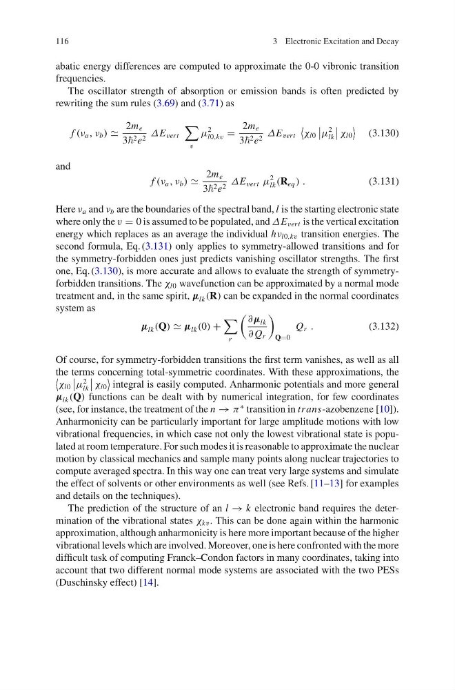
abatic energy differences are computed to approximate the 0-0 vibronic transition
frequencies.
The oscillator strength of absorption or emission bands is often predicted by
rewriting the sum rules (3.69) and (3.71) as
f (ν a , ν b )
2m e
3 2 e 2 ΔE ver t
v
μ
2
l0,kv =
2m e
3 2 e 2 ΔE ver t
χ l0
μ
2
lk
χ l0
(3.130)
and
f (ν a , ν b )
2m e
3 2 e 2 ΔE ver t μ
2
lk (R eq ) .
(3.131)
Here ν a and ν b are the boundaries of the spectral band, l is the starting electronic state
where only the v = 0 is assumed to be populated, and ΔE ver t is the vertical excitation
energy which replaces as an average the individual hν l0,kv transition energies. The
second formula, Eq. (3.131) only applies to symmetry-allowed transitions and for
the symmetry-forbidden ones just predicts vanishing oscillator strengths. The first
one, Eq. (3.130), is more accurate and allows to evaluate the strength of symmetryforbidden transitions. The χ l0 wavefunction can be approximated by a normal mode
treatment and, in the same spirit, µ lk (R) can be expanded in the normal coordinates
system as
µ lk (Q) µ lk (0) +
r
∂µ lk
∂ Q r
Q=0
Q r .
(3.132)
Of course, for symmetry-forbidden transitions the first term vanishes, as well as all
the terms concerning total-symmetric coordinates. With these approximations, the
χ l0
μ
2
lk
χ l0
integral is easily computed. Anharmonic potentials and more general
µ lk (Q) functions can be dealt with by numerical integration, for few coordinates
(see, for instance, the treatment of the n → π
∗ transition in trans-azobenzene [10]).
Anharmonicity can be particularly important for large amplitude motions with low
vibrational frequencies, in which case not only the lowest vibrational state is populated at room temperature. For such modes it is reasonable to approximate the nuclear
motion by classical mechanics and sample many points along nuclear trajectories to
compute averaged spectra. In this way one can treat very large systems and simulate
the effect of solvents or other environments as well (see Refs. [11–13] for examples
and details on the techniques).
The prediction of the structure of an l → k electronic band requires the determination of the vibrational states χ kv . This can be done again within the harmonic
approximation, although anharmonicity is here more important because of the higher
vibrational levels which are involved. Moreover, one is here confronted with the more
difficult task of computing Franck–Condon factors in many coordinates, taking into
account that two different normal mode systems are associated with the two PESs
(Duschinsky effect) [14].
3 Electronic Excitation and Decay
abatic energy differences are computed to approximate the 0-0 vibronic transition
frequencies.
The oscillator strength of absorption or emission bands is often predicted by
rewriting the sum rules (3.69) and (3.71) as
f (ν a , ν b )
2m e
3 2 e 2 ΔE ver t
v
μ
2
l0,kv =
2m e
3 2 e 2 ΔE ver t
χ l0
μ
2
lk
χ l0
(3.130)
and
f (ν a , ν b )
2m e
3 2 e 2 ΔE ver t μ
2
lk (R eq ) .
(3.131)
Here ν a and ν b are the boundaries of the spectral band, l is the starting electronic state
where only the v = 0 is assumed to be populated, and ΔE ver t is the vertical excitation
energy which replaces as an average the individual hν l0,kv transition energies. The
second formula, Eq. (3.131) only applies to symmetry-allowed transitions and for
the symmetry-forbidden ones just predicts vanishing oscillator strengths. The first
one, Eq. (3.130), is more accurate and allows to evaluate the strength of symmetryforbidden transitions. The χ l0 wavefunction can be approximated by a normal mode
treatment and, in the same spirit, µ lk (R) can be expanded in the normal coordinates
system as
µ lk (Q) µ lk (0) +
r
∂µ lk
∂ Q r
Q=0
Q r .
(3.132)
Of course, for symmetry-forbidden transitions the first term vanishes, as well as all
the terms concerning total-symmetric coordinates. With these approximations, the
χ l0
μ
2
lk
χ l0
integral is easily computed. Anharmonic potentials and more general
µ lk (Q) functions can be dealt with by numerical integration, for few coordinates
(see, for instance, the treatment of the n → π
∗ transition in trans-azobenzene [10]).
Anharmonicity can be particularly important for large amplitude motions with low
vibrational frequencies, in which case not only the lowest vibrational state is populated at room temperature. For such modes it is reasonable to approximate the nuclear
motion by classical mechanics and sample many points along nuclear trajectories to
compute averaged spectra. In this way one can treat very large systems and simulate
the effect of solvents or other environments as well (see Refs. [11–13] for examples
and details on the techniques).
The prediction of the structure of an l → k electronic band requires the determination of the vibrational states χ kv . This can be done again within the harmonic
approximation, although anharmonicity is here more important because of the higher
vibrational levels which are involved. Moreover, one is here confronted with the more
difficult task of computing Franck–Condon factors in many coordinates, taking into
account that two different normal mode systems are associated with the two PESs
(Duschinsky effect) [14].