

108
3 Electronic Excitation and Decay
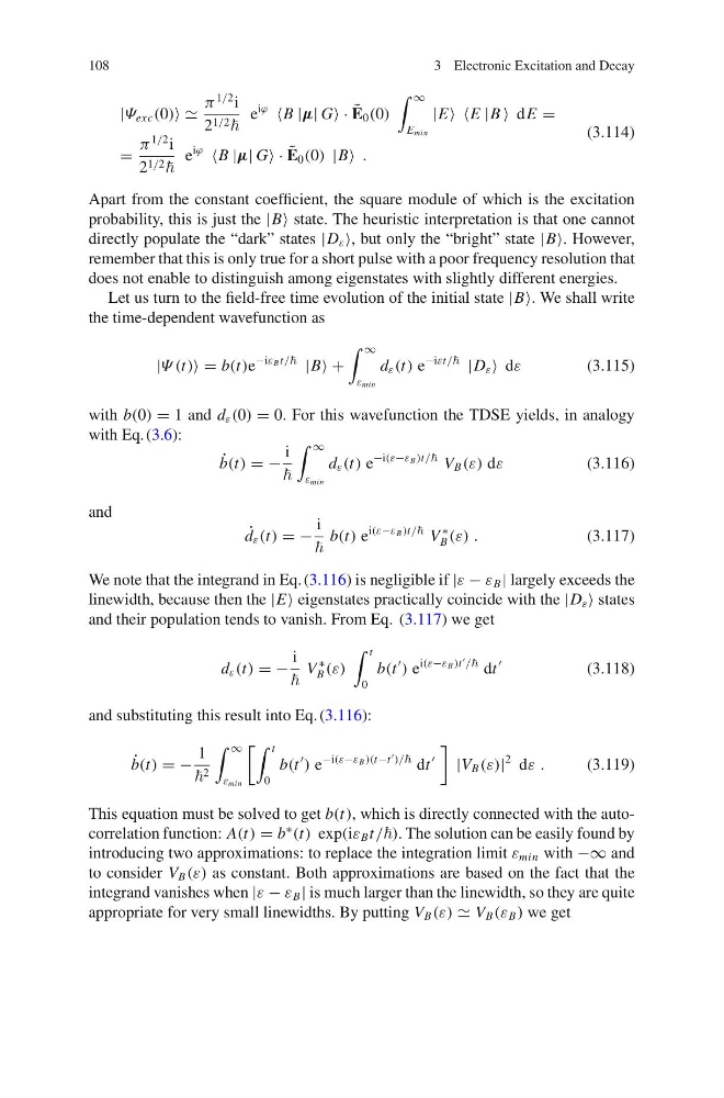
|Ψ exc (0)
π
1/2 i
2 1/2
e
iϕ
B |µ| G · ˜
E 0 (0)
∞
E min
|E E |B dE =
=
π
1/2 i
2 1/2
e
iϕ
B |µ| G · ˜
E 0 (0) |B .
(3.114)
Apart from the constant coefficient, the square module of which is the excitation
probability, this is just the |B state. The heuristic interpretation is that one cannot
directly populate the “dark” states |D ε , but only the “bright” state |B. However,
remember that this is only true for a short pulse with a poor frequency resolution that
does not enable to distinguish among eigenstates with slightly different energies.
Let us turn to the field-free time evolution of the initial state |B. We shall write
the time-dependent wavefunction as
|Ψ (t) = b(t)e
−iε B t/
|B +
∞
ε min
d ε (t) e
−iεt/
|D ε dε
(3.115)
with b(0) = 1 and d ε (0) = 0. For this wavefunction the TDSE yields, in analogy
with Eq. (3.6):
˙
b(t) = −
i
∞
ε min
d ε (t) e
−i(ε−ε B )t/ V B (ε) dε
(3.116)
and
˙
d ε (t) = −
i
b(t) e
i(ε−ε B )t/ V
∗
B (ε) .
(3.117)
We note that the integrand in Eq. (3.116) is negligible if |ε − ε B | largely exceeds the
linewidth, because then the |E eigenstates practically coincide with the |D ε states
and their population tends to vanish. From Eq. (3.117) we get
d ε (t) = −
i
V
∗
B (ε)
t
0
b(t
) e
i(ε−ε B )t
/ dt
(3.118)
and substituting this result into Eq. (3.116):
˙
b(t) = −
1
2
∞
ε min
t
0
b(t
) e
−i(ε−ε B )(t−t
)/ dt
|V B (ε)|
2 dε .
(3.119)
This equation must be solved to get b(t), which is directly connected with the autocorrelation function: A(t) = b
∗
(t) exp(iε B t/). The solution can be easily found by
introducing two approximations: to replace the integration limit ε min with −∞ and
to consider V B (ε) as constant. Both approximations are based on the fact that the
integrand vanishes when |ε − ε B | is much larger than the linewidth, so they are quite
appropriate for very small linewidths. By putting V B (ε) V B (ε B ) we get
3 Electronic Excitation and Decay
|Ψ exc (0)
π
1/2 i
2 1/2
e
iϕ
B |µ| G · ˜
E 0 (0)
∞
E min
|E E |B dE =
=
π
1/2 i
2 1/2
e
iϕ
B |µ| G · ˜
E 0 (0) |B .
(3.114)
Apart from the constant coefficient, the square module of which is the excitation
probability, this is just the |B state. The heuristic interpretation is that one cannot
directly populate the “dark” states |D ε , but only the “bright” state |B. However,
remember that this is only true for a short pulse with a poor frequency resolution that
does not enable to distinguish among eigenstates with slightly different energies.
Let us turn to the field-free time evolution of the initial state |B. We shall write
the time-dependent wavefunction as
|Ψ (t) = b(t)e
−iε B t/
|B +
∞
ε min
d ε (t) e
−iεt/
|D ε dε
(3.115)
with b(0) = 1 and d ε (0) = 0. For this wavefunction the TDSE yields, in analogy
with Eq. (3.6):
˙
b(t) = −
i
∞
ε min
d ε (t) e
−i(ε−ε B )t/ V B (ε) dε
(3.116)
and
˙
d ε (t) = −
i
b(t) e
i(ε−ε B )t/ V
∗
B (ε) .
(3.117)
We note that the integrand in Eq. (3.116) is negligible if |ε − ε B | largely exceeds the
linewidth, because then the |E eigenstates practically coincide with the |D ε states
and their population tends to vanish. From Eq. (3.117) we get
d ε (t) = −
i
V
∗
B (ε)
t
0
b(t
) e
i(ε−ε B )t
/ dt
(3.118)
and substituting this result into Eq. (3.116):
˙
b(t) = −
1
2
∞
ε min
t
0
b(t
) e
−i(ε−ε B )(t−t
)/ dt
|V B (ε)|
2 dε .
(3.119)
This equation must be solved to get b(t), which is directly connected with the autocorrelation function: A(t) = b
∗
(t) exp(iε B t/). The solution can be easily found by
introducing two approximations: to replace the integration limit ε min with −∞ and
to consider V B (ε) as constant. Both approximations are based on the fact that the
integrand vanishes when |ε − ε B | is much larger than the linewidth, so they are quite
appropriate for very small linewidths. By putting V B (ε) V B (ε B ) we get